ANSYS Beginner Truss Demo (draft 2, 11/20/05)

Start ANSYS and control colors

ANSYS is short for ANalysis SYStem. That pretty much sums up its capabilities.

Most areas of engineering calculation are included: stress, thermal, fluids, dynamics, vibrations, frequency analysis, acoustics, electromagnetism, optimization, etc. are present and usually have non-linear abilities as well. ANSYS was first released in 1971 and has generally been one of the most popular finite element systems since then, worldwide. Since it has a huge list of abilities its menu system can get relatively long. That is also true because it (and all FEA systems at that time) was run in a "batch mode" on the largest available computers. In other words, you could, and still can, execute ANSYS through an input text file without using a Graphical User Interface (GUI). Once you are fully experienced with the code that can be a real time saver. Every GUI session is saved in that format so that you can simply edit it with a text editor and make small changes for a similar problem.

Begin ANSYS with Start All Programs ANSYS 10.0 ANSYS. That will bring you to the main ANSYS Utility Menu:

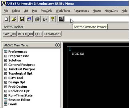
Figure Opening ANSYS to the Utility Menu and graphics window

If you utilize a black and white pri 434i820e nter you may wish to change the graphics background color (but that may hide some entities so their color needs changing also).

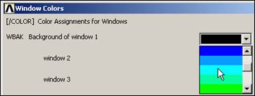
Figure Options for controlling colors in graphics

Select job name and analysis type

The various menus below will sometimes get moved to a back (hidden) window. If you think that has occurred hit the Raise Hidden button, . You will always need a job name:

1. Utility Menu File Change Jobname.
2. Change_Jobname, type in the new name, OK.

Figure Providing the required job name

The ANSYS files on real engineering problems get to be quite large, so have a directory dedicated to ANSYS:

1. Utility Menu File Change Directory.
2. Browse for Folder Change Working Directory, pick your directory (ANSYS_dir here), OK.

Figure Establish a directory for the analysis files

To keep up with your analysis studies over time create descriptive titles:

1. Utility Menu File Change Title.
2. Change Title, enter descriptive title, OK.

Figure Assign or change the analysis title

As the title suggests, this structure will be a planar truss. It will have three links that represent one (of two) end of a horizontal shelf which is intended to support a 1200 lb load. The shelf is 20 inches wide, and the vertical truss link will be 15 inches long. The top pin joint will support the weight on the shelf and will counter act the horizontal reaction, at the lower pin against the wall, which in turn balances the moment caused by the weight. You will neglect the weight of the truss itself here (but include it in your final design check).

Element type data

Since the problem class is that of a truss you will need a 2D structural line element, or link, that transmits only axial loads. Open and add to element types you need:

1. Main Menu Preferences Preferences for GUI Filtering.
2. Check Structural, accept default h-Method, OK.
3. Main Menu Preferences Element Type Add/Edit/Delete.
4. In Element Types pick Add Library of Element Types.
5. Select (Structural) Link and 2D spar 1, OK.
6. In Element Types pick Close.

Note that Link1 is 2D and by default is used only in the X-Y plane.

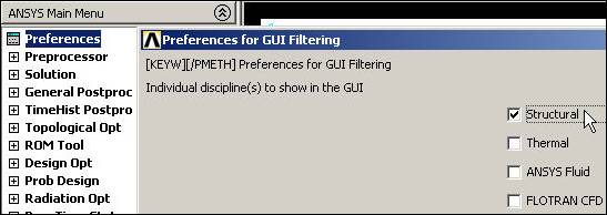
Figure Select the element type for the application

Element geometric properties data

Every element type requires one or more real constants, like area or moment of inertia, to describe it. Here, you simply need the cross-sectional area:

1. Main Menu Preferences Real Constants Add/Edit/Delete.
2. Real Constants Add Element Type for Real Constants.
3. Choose element type: Type 1 LINK1, OK.
4. Real Constant Set Number 1, for LINK1 verify Set No. 1,

Enter 0.125 for Cross-sectional area (AREA).

Enter 0 for initial strain (ISTRN), OK. Set 1 appears in Real Constants.

5. Select Add for the next element, verify Type 1 LINK1, OK.
6. Real Constant Set Number 2, for LINK1 verify Set No. 2,

Enter 0.35 for Cross-sectional area (AREA).

Enter 0 for initial strain (ISTRN), OK. Set 2 also appears in Real Constants.

7. Select Close.

XXX

Figure Providing the first real constant data set

Figure Adding an additional real data set

Define member material properties:

Here you will use the simplest linear, isotropic, 1D material description. ANSYS has full anisotropic (completely directionally dependent), as well as non-linear material "constitutive laws". Activate the material properties with:

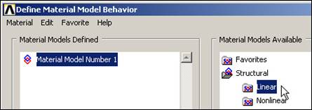
1. Main Menu Preprocessor Material Props Material Models.
2. Material Model Number 1 appears in Define Material Model Behavior.
3. Double click on Structural, then Linear, then Elastic, then Isotropic.
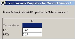
4. In Linear Isotropic Properties for Material Number 1 enter 3.e7 (psi) for isotropic elastic modulus, EX, and 0.27 for isotropic Poisson's ratio (PRXY), OK.
5. Define Material Model Behavior, Material New Model Define Material ID enter 2, OK.
6. Material Model Number 2 appears in Define Material Model Behavior.
7. Double click on Linear, then Elastic, then Isotropic.
8. In Linear Isotropic Properties for Material Number 2 enter 1.2e7 (psi) for isotropic elastic modulus, EX, and 0.3 for isotropic Poisson's ratio (PRXY), OK.
9. Close (X) the Define Material Model Behavior window.

Figure Select the material model behavior

Figure Provide isotropic data for the first material

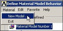
Figure Begin a second new material model

Figure Input isotropic properties for the second material

Define nodal data:

Of course, ANSYS has powerful mesh generation capabilities. However, for beginners or small problems with only a few nodes you can type in the coordinates, or use cursor input via the graphics window. Use the first approach:

1. Main Menu Preprocessor Modeling Create Nodes In Active CS.
2. In Create Nodes in Active Coordinate System enter 1 for Node number, X = 0., Y = 0., default Z to zero (2D LINK1 element does not use it), Apply, enter 2 for Node number, X = 20., Y = 0., Apply, enter 3 for Node number, X = 0., Y = 15., OK.
3. If you make a mistake you can return and correct it in the above window, or delete them all with Preprocessor Modeling Delete.

Figure Manually create the first node and its coordinates

Now, plot the nodal values input (here node 1 is hidden behind the axis symbol):

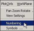
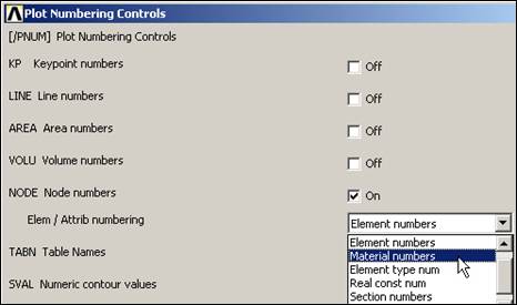
1. Utility Menu PlotCtrls Numbering.
2. In Plot Numbering Controls check node numbers and select element numbers in the pull down menu, OK.
3. Utility Menu PlotCtrls Numbers and review the plot.

Define element attributes

Next you have to associate each of the elements with your previous material numbers and real constant sets. Plan ahead and input those of the same type in sequence:

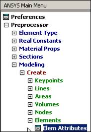
1. Main Menu Preprocessor Modeling Create Elements Elem Attributes.
2. In Element Attributes select defaults (type number = 1, material number = 1, real constant set = 1), OK.
3. Main Menu Preprocessor Modeling Create Elements Auto numbered Thru Nodes.
4. In Elements from nodes verify that Pick is checked on.
5. In the graphics window define the first element by picking node 1 (a square symbol appears) then node 2, OK, and the next element number (1) appears.

Figure Prepare for node and element plots

XXX

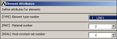
Figure Associate data attributes with each element group

The next element two elements have different attributes (material number) from the first element. In a similar fashion define them with

1. Main Menu Preprocessor Modeling Create Elements Elem Attributes.
2. In Element Attributes keep default type number (1), change material number to 2, real constant set to 2, OK.
3. The next element has the same attributes, so just input its connectivity. Click on Thru Nodes again, pick node 2 then node 3, OK, so element 2 appears.
4. Repeat for element 3.

Check mesh data

It is wise to check such manual input by plotting the nodes and elements via:

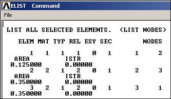
1. Utility Menu List Elements Nodes+Attr+RealConst.
2. When the ELIST (ELement LIST) window appears check those data and close it.

Figure Checking the mesh graphically and with a list

Apply displacement restraints

The displacement restraints must be applied to reflect the physical support (often the most unclear part of an analysis) as well as eliminating all the "rigid body motions" (RBM). Here there are two translational RBM plus a rotation about the normal (Z) axis. Apply them via:

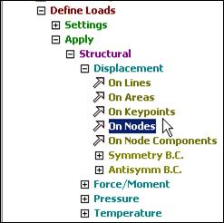
1. Main Menu Preprocessor Loads Define Loads Apply Structural Displacement On Nodes.
2. In Apply U, Rot on Nodes verify that Pick and Single are checked on, in the graphics window, select top node 3 (for vertical and horizontal restraints), OK. After the panel changes form, highlight the horizontal (UX) and vertical (UY) components as the degrees of freedom (DOF) to be constrained.

Figure Beginning the nodal displacement restraints at a picked node

3. Under Constant value enter 0, OK.
4. Click on On Nodes again and pick node 1 to be restrained in the horizontal (UX) direction with a Constant value of 0.

Figure Nodal displacement restraint at the second picked node

Note that these restraint operations are shown in the graphics window as triangles pointing in the direction of restraint, at each restrained node.

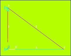
Figure Graphical spot check of mesh and restraints

To list the current restraints:

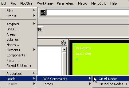
1. Utility Menu List Loads DOF Constraints On All Nodes.
2. When the (Displacement LIST) DLIST window appears check those data and close it.

Apply nodal loads

This shelf is intended to carry a total loan of 1200 lb. Half of that must go to the two lower nodes on each end. Since a Link1 element is a "two force member" and a truss transmits forces at the nodes via "concurrent forces" you are not allowed to specify a load at the center edge of the shelf (that is, at the center of element 1). To do that you would have to select an element type with bending resistance. Instead, you will attach the shelf at the two horizontal nodes. Each carries half (300 lb) of the truss's share of the load. Specify that with:

Main Menu Preprocessor Loads Define Loads Apply Structural Force/Moment On Nodes.

2. In Apply F/M on Nodes verify that Pick and Single are on, and then pick node 1 and also node 2, OK.
3. When the window changes form, pick a vertical force (FY) for the Direction of force and -300 (lb) for the Constant value, OK.

Figure Checking the displacement constraints list

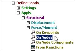
Figure Applying joint forces with a nodal pick

Note that these load operations are shown in the graphics window as arrows pointing in the direction of load, at each restrained node. If your plot does not show everything you have defined also try PlotCtrls Symbols. Symbols and check that the items you want are turned on.

Figure Graphics window check of joint loads

To list the current loads:

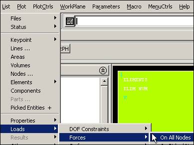
1. Utility Menu List Loads Forces On All Nodes.
2. When the Force LIST (FLIST) window appears check those data and close it.

Figure List the joint forces for checking

Figure Add the restraints and their future reactions to the plot symbols

Saves and restarts

At this point you may want to save your data to go to class and restart the actual analysis later. If so:

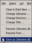
1. Utility Menu File Save as Jobname.db.
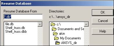
2. Upon return open ANSYS and enter Utility Menu File Resume from. to get the list of your ANSYS database (db) files so you can select the one you want.

Figure Typical save and restart options

Solve for displacements and secondary variables

To use the current (and only) load system (LS) enter:

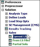
1. Main Menu Solution Solve Current LS, review the listed summary, OK.
2. When the solution of the simultaneous equations is complete you will be alerted that the solution is done.

Figure Starting the displacement solution for this load case

Post-processing

Displacements

It is always wise to visually check the computed displacements:

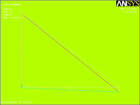
1. Main Menu General Postproc Plot Results Deformed Shape.
2. In Plot Deformed Shape pick the combined deflected and undeformed option for the Items to be plotted (KUND), OK. Check the plot in the graphics window.
3. Animate the computed deflections with:Utility Menu PlotCrtls Animate Deformed Shape.
4. Pick Def+undeformed in Animate Deformed Shape, OK.
5. If desired, employ the Animation Controller that appears, or simply pick Stop, Close.

Figure Undeformed and deformed structure

To create a hardcopy (you may need to try various background colors):

Utility Menu PlotCrtls Hard Copy Printer (or File), select your printer name, Print.

Figure Sending the current plot to the printer or a file

To see a (potentially long) list of displacement results:

1. Preferences General Postproc List Results Nodal Solution.
2. In List Nodal Solution Nodal Solutions DOF Solution Displacement vector sum, OK.
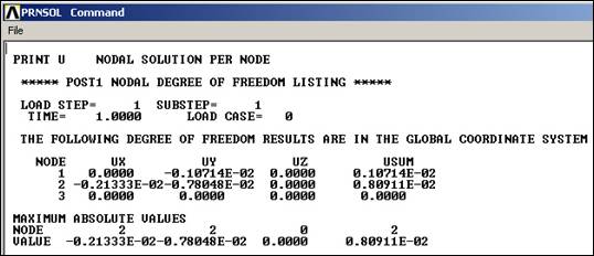
3. Examine the results in the PRNSOL (PRint Nodal SOLution) Command window and close it.

Figure List the nodal displacement vector components

Reaction Forces

If the solver does not fail then your reactions will be equal and opposite of your resultant forces and moments. Therefore they let you check the level of loads actually applied, versus what you intended to apply. That is helpful especially for pressure loads. Check them with:

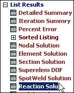
1. Main Menu General Postproc List Results Reaction Solution.
2. In List Reaction Solution pick All items for Item to be listed, OK.
3. Review the Print Reaction SOLution (PRRSOL) Command window.

Figure List reaction forces associated with displacement restraints

Notice that the vertical reaction force of 600 (lb) is equal and opposite to the sum of the applied loads. Likewise, there were no horizontal forces applied, so the top (400 lb) and bottom (-400 lb) wall reactions yield a null horizontal force. They also form a couple (of 400 lb * 15 in = +6,000 in-lb) that is equal and opposite to the moments of the applied forces (of 0 - 300 lb * 20 in = -6,000 in-lb), relative to node 1.

Member forces

The element (member) forces in the truss resulting from the computed displacements can also be recovered and listed (along with entities such as elastic and thermal strains that are not considered here) with:

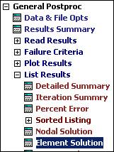
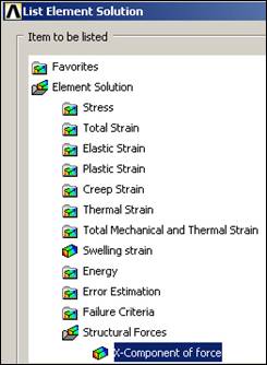
1. Main Menu General Postproc List Results Element Solution.
2. Get the member axial forces, in global components, from List Element Solution Element Solution Structural Forces, OK.
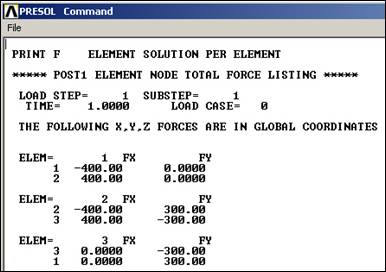
3. Review the PRESOL (PRint ELement SOLution) Command display and close the window.

Figure Recover the global component of member axial forces

Generally, for trusses and frames (1D elements in 2D space) you need to see the force results in the local (member) coordinate components. They are seen with:

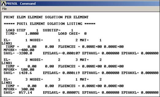
1. List Element Solution Element Solution Line Element Results.
2. There you are mainly interested in the axial Member FORce X-direction (MFORX) values (in lb) and the Stress in the AXiaL direction (SAXL), in psi, but not currently in other items like the strain ( , or EPsilon) of the ELement in the AXiaL direction (EPELAXL). The MFORX is negative for compression (consider buckling there) and positive in tension.

Figure List the local (member) coordinate components of element entities

(JEA stress levels SAXL seem low here, double check data, XXX)

Exiting ANSYS

You can save the results to your data base, as described above, and close with File Exit.

To begin a different analysis, instead of picking Exit, use File Clear & Start New ., OK.

(end)