The purpose of this exercise is to cover the basic functionality of the Mechanical Toolbar (MTB) in the context of performing an actual analysis. Details of each command, along with an explanation of why you are using the command, are provided prior to each step.
This will be a simple problem that will be performed entirely within the MTB to give the student a quick overview of the MTB functionality. This exercise will use the very minimum of input required to progress through the steps and obtain results. The model will employ the no defeature/repair option during import of a solid 3D part, MTB materials, Smartsize meshing, simple area constraints, and area force loading.
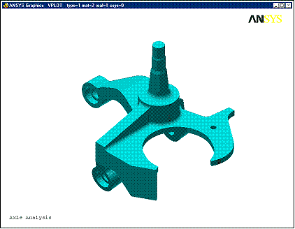
The analysis will be performed on a 3-D solid model of an automobile front wheel axle. The model has already been sufficiently defeatured to facilitate building the finite element model. You will use the MTB to determine maximum stress and deflection and if the axle can withstand the given loads without yielding.
Important: Please Read the Following
This exercise contains the step by step instructions to complete the problem described above. All instructions to the exercise are denoted by Blue colored text.
This exercise also contains detailed information about the functions on Mechanical Toolbar. The information that is provided covers the required functions necessary to complete this exercise. Other functions will be covered in later exercises. The information should be read before proceeding with the instructions. The detailed information is denoted by the Black colored text.
 |
Launch ANSYS/Professional With The MTB:
Launch ANSYS.
Activate Mechanical Toolbar
Setup:
Engineering Discipline.
Analysis Type
Unit System
Graphic Title
Toolbar Properties
Model:
Model Preparation
Importing Models
Viewing The model
Material Properties
Meshing the Model with SmartSizing
The Mesh Tool
Loads And Boundary Conditions:
Environment
Adding or Deleting Loads and B.C.'s
Solve:
Solve Now
Solve Later
Linear Elastic Solution Results
Results Item
Results Display
Reports
Conclusion
Additional Functions
Create a folder on your computer for this job and copy the parasolid file axle.xmt_txt to this folder from the InputFiles folder on the CD.
If you do not have a parasolid translator, copy the file axle.db instead. When you reach section 3.2 (Import Model), select ANSYS (*db*) for type of file and import the axle.db file.
Launch ANSYS/Professional and Activate the Mechanical Toolbar (MTB)
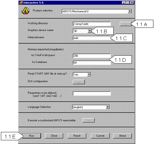
Launch ANSYS using your start menu.
A. Browse to select the working directory you just created for this job.
B. Change the Graphics device name to 3D
C. Enter a job name (axle). All ANSYS files created for this problem will have a filename of axle followed by a unique extension.
D. Change the Memory Requested for Total Workspace and for Database sizes for this job to be 256 and 64 respectively.
E. Click RUN to start the ANSYS GUI.
The following step is required only if you are not running ANSYS Professional.
Activate the Mechanical Toolbar (MTB).
A. Click on MenuCtrls
B. 
Click on Mechanical Toolbar. The Mechanical Toolbar (MTB) will now
appear and replace the Main Menu, Input Window, and the Toolbar.

By default the MTB will first display the Setup tab. This is where you will specify the analysis
settings. The MTB options will vary
depending on which Tab is currently active.
Setup
On the Setup tab, you are required to specify the engineering discipline, analysis type, unit system, and the graphics title for the analysis. You also have options for setting your MTB preferences and inputting user information.
Set the Engineering Discipline

To set the engineering discipline, click on the Engineering Discipline drop
down list and select either Structural or Thermal. The selected option will directly affect
which options are presented to you in the Analysis
Type drop down list.
A. Set the Engineering Discipline to Structural
Analysis Type

To set the analysis type, click on the Analysis Type drop down list and select
the type. If the Engineering Discipline is set to Structural, you have the options of either Static or Modal. If the Engineering
Discipline is set to Thermal,
then you only have the option of Steady-State.
A. Set the Analysis Type to Static
Unit System

To set the unit system, click on the Unit System drop down list and select the
unit system that you want to work in. You also have the option to define a new unit system. The unit system that you choose has no effect
on existing data or completed analyses. It is only used to define labels on the plots for
convenience. If you change units during
the modeling process, ANSYS does not perform a unit conversion for you. That is your responsibility. Be consistent with your units.
The unit system options include:
m-kg-sec-°C
cm-g-sec-°C
foot-slug-sec-°F
inch-lbm-sec-°F
mm-kg-sec-°C
Add Unit System
A. Set the Unit System to m-kg-s-°C
Graphic Title

To name the analysis, click in the Graphic Title input window, delete the default
name (ANSYS Analysis), and type in the new name. You are allowed up to 72
alphanumeric characters.
A. Enter a Graphic Title for the analysis: Axle Analysis.
Toolbar Properties

![]() Toolbar
Properties button contains options to allow you to affect the behavior of the
MTB. To modify these options, click on
the Toolbar Properties button. Three tabs appear on the dialog box: General,
User Info, and About.
Toolbar
Properties button contains options to allow you to affect the behavior of the
MTB. To modify these options, click on
the Toolbar Properties button. Three tabs appear on the dialog box: General,
User Info, and About.
Click the General tab to change the start-up configuration of the MTB, to define a system calculator or system editor, or to enable PostScript printing. (for Windows NT systems only)

If the *ABBR Toolbar or the Input Window has been turned off via the
MenuCtrls in the full ANSYS menu
system, you must turn off the Mechanical Toolbar and then turn it back on after
choosing either of these configuration options from the Toolbar Properties
dialog box. Otherwise, they will not appear in the interface.
Toggling ON the *ABBR Toolbar allows you to
access the ANSYS GUI component known as the *ABBR Toolbar. This toolbar
contains a set of push buttons that execute commonly used ANSYS functions. You can
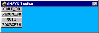
customize this toolbar by adding or removing functions.

Toggling on the Input Window allows
you to access the ANSYS GUI component known as the Input Window. Using this
window, allows you to input commands directly to ANSYS.

![]() The
System Utilities-Calculator allows
you to input the name of your preferred system calculator in the text entry
box. The MTB will start the defined calculator when you click the System
Calculator button on the MTB.
The
System Utilities-Calculator allows
you to input the name of your preferred system calculator in the text entry
box. The MTB will start the defined calculator when you click the System
Calculator button on the MTB.
![]() The
System Utilities-Editor allows you
to input the name of your preferred system text editor. The Mechanical Toolbar
will invoke the defined editor when you click the System Editor button on the
MTB.
The
System Utilities-Editor allows you
to input the name of your preferred system text editor. The Mechanical Toolbar
will invoke the defined editor when you click the System Editor button on the
MTB.
The System Utilities-Enable PS print (Windows NT systems only). Check this box if you are using a PostScript-enabled printer for better print quality.

Click the User Info tab to provide
user information for Analysis. You can record your name, company name, and
company address in the corresponding text entry boxes. The Mechanical Toolbar
uses these entries when creating the report.
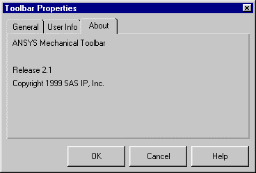
Click the About tab to verify which
version of the Mechanical Toolbar you are using. Just in case you forgot.
To put your changes into effect and exit the Toolbar Properties dialog box, click OK. To put any Start Configuration changes into effect, you must also restart the Mechanical Toolbar.
A. 
![]() Click
on the Toolbar Properties button.
Click
on the Toolbar Properties button.
B.
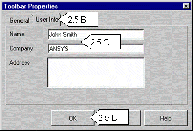
The Toolbar Properties dialog will appear. Click on the User Info tab.
C. Enter your name, and if you want, company name and address.
D. Click OK when finished.
Model
Under the Model tab is where you import the geometry, assign shell element thickness, material properties and mesh the part.

With the MTB you do not have the capability to create the volumes or areas,
therefore the geometry must be imported.
Model Preparation
The following are a few tips on how to prepare the geometry before importing it into ANSYS.
Create a copy of the model in your CAD system. Modify the copy by simplifying the geometry to better facilitate the building of the finite element model.
Suppress unnecessary features in the model such as external fillets, small holes, and any feature that is not essential to the analysis.
Cut the model on all symmetry planes. Only keep the smallest unique piece that can be mirrored or copied (note that the loads and boundary conditions must also be symmetric).
Remove or suppress everything from the model that isn't part of the model's geometry, such as dimensions, construction lines, etc.
Either move the model near the geometric center of the coordinate system or create an output coordinate system near the geometric center of the model.
Analyze the model and look for any small slivers or poor geometry. Remove these areas or correct the geometry.
Importing Models

![]() To
load a model into the Mechanical Toolbar, click the Import Geometry button. The Import Geometry - Select File dialog
will appear.
To
load a model into the Mechanical Toolbar, click the Import Geometry button. The Import Geometry - Select File dialog
will appear.
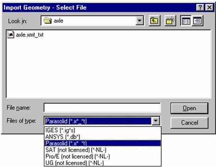
Click on the Files of type drop down
list and select one of the import types.
Change the directory to the directory containing the file to be imported.
Highlight the desired file name and click Open. The Import Geometry - Select Import Method dialog will appear.
If you do not have a parasolid translator, copy the file axle.db instead. When you reach section 3.2 (Import Model), select ANSYS (*db*) for type of file and import the axle.db file.
Use the Import
Geometry - Select Import Method dialog box to decide which method to use when
importing a model. Specify whether the
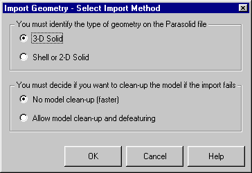
model is a 3-D Solid or a Shell or 2-D Solid.
You have two additional choices to make concerning your model
No model clean-up - This is the preferred method; it's faster and more reliable.
Allow model clean-up and defeaturing - Using this method activates the defeaturing tools. A better method is to remove all unnecessary features from your model in the CAD system.
Click OK to proceed with the geometry import.
A. 
![]() Import
the geometry for this exercise. Click on
the Model tab on the MTB.
Import
the geometry for this exercise. Click on
the Model tab on the MTB.
B. Click on the Import geometry button to bring up the Import Geometry - Select File dialog box.
C.

Change the Files of type: option to Parasolid.
D. Change the directory to the directory containing the axle parasolid.
E. In the file list, highlight the file named axle.xmt_txt.
F.
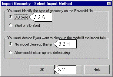
Click Open. The Import Geometry - Select Import Method dialog will
appear
G. Select 3-D Solid.
H. Leave the No model clean-up (faster) option set.
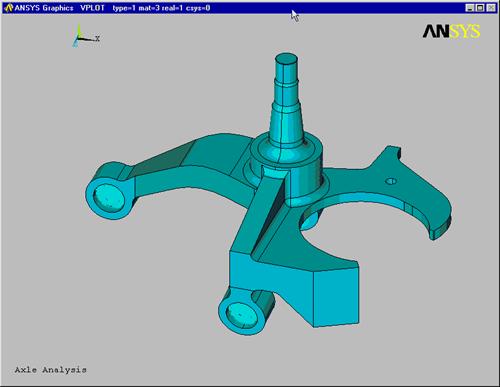
I. Click OK. ANSYS will import the Parasolid file and draw the part in the graphics window.
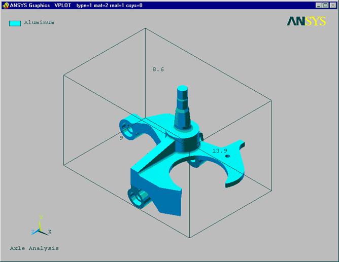
Viewing the model

There are several buttons on the Mechanical Toolbar that allow you to
manipulate graphic plots. These buttons and their functions include:
![]() Plot: To access a fly-out toolbar of
plotting options, do the following:
Plot: To access a fly-out toolbar of
plotting options, do the following:
![]()
Position the cursor on the Plot button.
Press and hold the left mouse button until the fly-out toolbar appears.
The fly-out toolbar contains the following buttons: Keypoint Plot, Line Plot, Area Plot, Volume Plot, Node Plot, and Element Plot.
Release the left mouse button.
![]() Position the cursor on the desired fly-out button and
click.
Position the cursor on the desired fly-out button and
click.
![]() Oblique View: Sets the view of the
graphic window to oblique.
Oblique View: Sets the view of the
graphic window to oblique.
View: Sets the view of the graphic window. To access a fly-out toolbar:
Position the cursor on the View button.
![]()
Press and hold the left mouse button until the fly-out toolbar appears.
The fly-out toolbar contains the following View option buttons: Top View, Bottom View, Front View, Back View, Left View, Right View, Oblique View, Working Plane View, and Isometric View.
![]()
 Pan-Zoom-Rotate:
This option activates the Pan-Zoom-Rotate control, which allows you manipulate
the model view by panning, zooming, or rotating the model. Note:
This is a good option to leave on while working on the model.
To change the view, click on the desired view button (Top, Front, Iso, etc)
You can choose a Zoom method. Your options include: Zoom, Box Zoom, Win Zoom, and Back Up (UnZoom).
Pan/Zoom buttons: Pan up/down left/right using the arrows. Small dot zooms out and the large dot zooms in. The Rate slider located below the rotate buttons controls the amount of change in model size from zooming in or out.
The Rotate buttons allow you to define the axis of rotation. The rate slider that is below the rotate buttons controls the amount of rotation.
Dynamic Mode: This option allows you to use your mouse buttons to pan/zoom/rotate. When this is on, the left mouse button pans, the middle mouse button zooms, and the right mouse button rotates.
Lighting: This option allows you to control the light source location, intensity, and the reflectance of your model. When this option is ON the mouse buttons function as follows: Left Button: Move in X-direction to increase or decrease the reflectance of your model. Move in the Y-direction to change the intensity of the directional lights (there are two directional lights, one in front and one behind your model). Middle Button: Move in the X-direction to rotate the directional lights about the screen Z-axis. Move in the Y-direction to change the intensity of the ambient light. Right Button: Move in the X-direction to rotate the directional lights about the screen Y-axis. Move in the Y-direction to rotate the lights about the screen X-axis.
Fit: Automatically adjusts that amount of zoom in the active window so that your entire model can be seen within the window.
Reset: Removes any Pan-Zoom-Rotate changes in the active window. Your model will be displayed in its default orientation and sized to fit within the active widow.
Close: Dismisses the Pan-Zoom-Rotate dialog box.
Alternatives to using the Pan-Zoom-Rotate control
Pan - Hold down the CTRL key and press the left mouse button. Move the mouse left, right, up, or down to move the model in the desired direction.
Zoom - Hold down the CTRL key and press the middle mouse button. Move the mouse up to zoom in. Move the mouse down to zoom out. If you are using a two-button mouse, you may be able to mimic the action of a middle mouse button by holding down the SHIFT key and pressing the right mouse button.
Rotate about Z axis - Hold down the CTRL key and press the middle mouse button. Move the mouse left or right to rotate the model about the Z axis. If you are using a two-button mouse, you may be able to mimic the action of a middle mouse button by holding down the CTRL-SHIFT keys and pressing the right mouse button.
![]() Rotate about X or Y axis-Hold down the CTRL key and press the right mouse
button. Move the mouse to rotate the model about the X (up/down) or Y
(left/right) axis.
Rotate about X or Y axis-Hold down the CTRL key and press the right mouse
button. Move the mouse to rotate the model about the X (up/down) or Y
(left/right) axis.
Redraw Model: Redraws (refreshes) the contents of the graphic window.
![]() Render Model: This option allows you to
set the render options for the model. The render options include material
coloring, material texturing, thickness, translucency, wireframe, gray scale,
and show edges.
Render Model: This option allows you to
set the render options for the model. The render options include material
coloring, material texturing, thickness, translucency, wireframe, gray scale,
and show edges.
Boundary Conditions: Toggles boundary condition symbols on and off.

![]() Print
Hardcopy: Prints a hardcopy of the graphic window contents.
Print
Hardcopy: Prints a hardcopy of the graphic window contents.
A. Select
the Pan-Zoom-Rotate button. The Pan-Zoom-Rotate dialog will appear ![]()

B. Thoroughly inspect the model by Panning, zooming, and rotating the model. Play with the light source option.
C. ![]()

Return the view to Oblique when you
are finished. Leave the Pan-Zoom-Rotate
control open for the rest of the exercise.
![]()
Material Properties
By default, there are three materials that are available for use with the Mechanical Toolbar: these are ANSYS-supplied aluminum, steel, and titanium. In addition to these ANSYS-supplied materials, you can add other materials to create your own personal material library.
To create a new material that will be added to your personal material library, you need to be on the Model tab. Follow these steps:
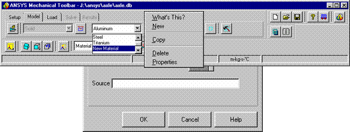
Click on the Default Material drop
down list and select New Material,
or place the cursor over the Default
Material drop down list, click the right mouse button and select New from the list of options. The Material Properties dialog box appears.
Three tabs appear on the dialog box: Display, Structural, and Thermal.
On the Display tab, type a unique name for the new material into the Name window. Material names are limited to 32 characters.
Click on the arrow to the right of the Material Texture button. When the texture options appear, click the texture of your choice to select it. The Mechanical Toolbar will use the texture that you choose to depict the material in graphic plots.
Use the Source input window to record information about the source that you referred to for the definition of the material (up to 64 characters, including spaces).

Click on the Structural or Thermal tab (as applicable) and type in
the physical constants that are necessary to define the new material.
Click OK to put your changes into effect and exit the Material Properties dialog box. The new material will be added to your personal material library and will always appear in the Default Material drop down list box on your system.
Place the cursor over the Default Material drop down list, click the right mouse button and select Copy, Delete, or Properties.

Any unassigned model entities will take on the material that is currently
displayed in the Default Material drop down list. To assign a material to
entities in a model, you need to be on the Model tab. Follow these steps:
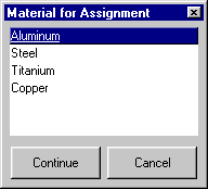
![]() Click on the Assign Material button. The Material for Assignment dialog will
appear.
Click on the Assign Material button. The Material for Assignment dialog will
appear.
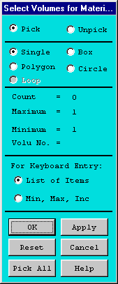 In
the Material for Assignment dialog
box, select the desired material and then click Continue. The ANSYS Picker
will appear.
In the picker, make the desired picker selections (for example, Single pick, Box pick, and so on).
In the graphic window, select those parts of the model to which you want to assign the material.
Click Apply in the picker.
Repeat steps 1 through 5 until you have assigned a material to all appropriate entities in the model.
Click OK in the picker.
A. ![]() Next
we want to change the material properties from the default of
Next
we want to change the material properties from the default of 
Aluminum
to Steel. Click on the Assign Material button in the MTB.
B. 
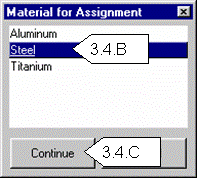 ANSYS has built in properties for Aluminum,
Steel and Titanium. Highlight Steel in the list.
C. Click Continue.
D.
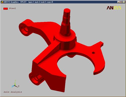
The picker dialog will appear for you
to select volumes for material assignment. Click the button that says Pick
all. The plot will change to reflect the change in material.
Meshing the model with Smart Sizing
Meshing the model is performed on the Model tab.

Click on the Mesh SmartSize slider and move it from left (fine mesh) to right
(coarse mesh) to define the overall element size for the mesh. As you move the
Mesh SmartSize slider, notice that the Mesh Model icon that appears to the
right of the slider changes in size as you move the slider.
You can use Smart Sizing to set different mesh sizes for different parts of a model. To do so, set a Smart Sizing level and mesh only those entities in the model that should have that level. Then continue setting levels and meshing entities (one or more entity at a time), until all entities in the model are meshed.
![]() Set
the level of the Smart Size by moving the slider either to the left or the
right, then select the Mesh Model button.
Set
the level of the Smart Size by moving the slider either to the left or the
right, then select the Mesh Model button.
![]()
 The MeshTool provides access to more advanced
meshing controls and meshing operations.
Element Attribute Controls on the MeshTool are ignored when the Mechanical Toolbar is active.
Clicking the Smart Size check box toggles SmartSizing on and off. This option is identical to SmartSizing on the Mechanical Toolbar's Model tab.
Global: Controls the setting and clearing of global element edge lengths.

Clicking Set opens a dialog box for
setting the global edge length
Clicking Clear clears this specification.
Areas: Controls the setting and clearing of element edge lengths on selected areas.
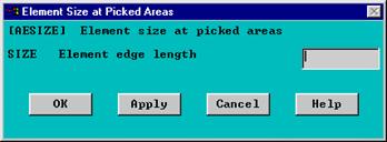
Clicking Set opens a picking dialog
for selecting areas, followed by a dialog box for setting element edge lengths
on the selected areas
Clicking Clear allows you to select areas and clear this specification.
 Lines:
Controls the setting and clearing of the divisions and spacing ratios on
selected unmeshed lines.

Clicking Set
opens a picking dialog for selecting lines, followed by a dialog box for
setting divisions.
Clicking Clear opens a picking dialog for selecting lines to be cleared of divisions.
Clicking Copy opens a picking dialog to let you copy line divisions (including spacing ratios) from one line onto other unmeshed lines. First, pick the line from which divisions will be copied, then click OK in the picking dialog. Next, pick the lines to which the divisions should be copied, then click OK in the picking dialog. If previously set line divisions exist, the copied divisions overwrite them.
Clicking Flip opens a picking dialog to let you flip the spacing ratio of line divisions (from one end to the other) on an unmeshed line. First pick the line to be flipped, then click OK in the picking dialog.
Layer: Layer meshing is used in the modeling of fluid flow. It is not of use to Mechanical Toolbar users.
Keypts: Controls the setting and clearing of the edge lengths of the elements near a selected keypoint or keypoints. Clicking Set opens a picking dialog for selecting keypoints, followed by a dialog box for setting edge lengths. Clicking Clear opens a picking dialog for selecting the keypoints for which you wish to clear the keypoint sizing specifications.
Mesh: Controls which type of entity is being meshed. For Mechanical Toolbar users, only Volumes (for solids) and Areas (for shells and planes) are valid choices.
 Shape:
Controls the shape of the elements used to create a mesh (quadrilateral,
triangle, hexahedral, or tetrahedral). Mechanical Toolbar users should leave
this control set to Tet when meshing volumes, and Quad when meshing areas.
Mesher: Controls which type of meshing (free or mapped) is used to mesh a model. Mechanical Toolbar users should leave this control set to Free for both volume and area meshing.
![]() Mesh: Starts the meshing operation.
Clicking Mesh opens a picking dialog that lets you select the entity to be
meshed. You can also start a meshing operation by clicking the Mesh Model
button on the Model tab of the Mechanical Toolbar.
Mesh: Starts the meshing operation.
Clicking Mesh opens a picking dialog that lets you select the entity to be
meshed. You can also start a meshing operation by clicking the Mesh Model
button on the Model tab of the Mechanical Toolbar.
Clear: Clears the selected volumes, areas, lines, and keypoints (i.e., vertices) of their meshes. Clicking Clear opens a picking dialog that lets you select the entity to be cleared.
Refine at: Controls the general location at which mesh refinement occurs. Clicking the drop down list box causes a list of available choices-Nodes, Elements, KeyPoints, Lines, Areas, and All Elems-to appear.
Refine: Starts the refinement operation. Clicking Refine opens a picking dialog box that lets you select the specific area(s), line(s), etc. at which you want refinement to occur.
Meshing: We will use the default SmartSize meshing to create a mesh on the part. The resultant mesh will be good enough to run the preliminary analysis.
A. The slider bar in the MTB controls the SmartSize mesh density in various levels from very fine (left most setting) to very course (right most setting). We will use the default (center setting).
B. Since there is only 1 volume in the model, click on the Mesh Model button to create the mesh. The ANSYS meshing process may take a few minutes. When meshing is complete, the mesh will appear in the graphics window.
C. 
Take a look at the nodes. In the MTB,
click and hold on the Plot button
momentarily until the fly-out options appear.
D.
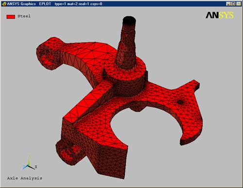
Click on the Plot Nodes Button. Notice that the Render Model option has changed to Show Edges.
E. 
Click on Render Model. Try some of the other Render Model
options. Return to Material Coloring when you are finished
F. Click and hold on the Plot Button and pick Plot Elements.
Loads and Boundary Conditions

Now that we have completed the model definition phase, it's time to apply the
loads and boundary conditions.
Environment
An environment is a set of boundary conditions (loadcases) applied to the model. You are allowed to define multiple environments. This is useful when you want to examine and compare the behavior of the model under different loads or boundary conditions.

The MTB allows you to add, copy, rename, or delete an environment.
To create a new environment and assign a name, perform the following:

Select the New Environment... option
from the Load Environment drop down list box, or Right-click the mouse while it
is positioned over the Load Environment drop down list and click on New. The New Environment dialog box appears.
Type the name of the new environment. Names are limited to 32 characters.
Click OK. The new environment name now appears in the list of existing environment names.
To copy an existing environment to a new environment, perform the following:
 Select the Copy Environment... option from the Load Environment drop down list
box. The Copy Environment dialog
appears.

Select the environment to be copied in the From window, and type in the new
environment name in the To window.
Click OK
To delete an environment perform the following:
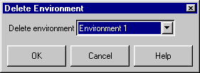
 Select the Delete Environment... option from the Load Environment drop down
list box. The Delete Environment
dialog appears.

Select the environment to be deleted and click OK.
To Rename an environment perform the following:

 Select the Rename Environment... option from the Load Environment drop down
list box. The Rename Environment
dialog appears.

Select the environment to be renamed.
Type in a new name and click OK.
Adding or Deleting Loads and Boundary Conditions

![]() In
the Mechanical Toolbar, you specify whether you want to add or delete a load
before selecting the specific type of load. Click the Add B.C. or the Delete B.C. button, and then click the
button representing the load type you want to add or delete.
In
the Mechanical Toolbar, you specify whether you want to add or delete a load
before selecting the specific type of load. Click the Add B.C. or the Delete B.C. button, and then click the
button representing the load type you want to add or delete.
Make sure the proper Environment is set prior to creating a load or boundary condition.
After you click on a load type button, a picker appears that allows you to select the entity to which you are applying the load, or from which you are deleting the load.
To create boundary conditions
Choose the environment for which this B.C. applies.
Click the Add B.C. button.

Select Constraint to remove one or more degrees of freedom from the selected object type.

With the cursor positioned on the Constraint
button, hold down the left mouse button. A fly-out toolbar appears. You can
constrain a keypoint, a line, or an area.
Click on the button representing the entity constraint you want.

A picker appears. Select the keypoints, lines,
or areas to be constrained. Click OK.
A Constrain dialog box appears.
Select the direction(s) in which you want to constrain the model.
Select the coordinate system you want to use to specify the direction if other than the default Global Cartesian system.
Click OK.

Select Fixed to remove all degrees of freedom from the selected object type.
![]()
With the cursor positioned on the Fixed
button, hold down the left mouse button. A fly-out toolbar appears. You can fix
a keypoint, a line, or an area.
Click on the button representing the entity you want to fix.
A picker appears. Select the keypoints, lines, or areas to be fixed.
Click OK.
Apply the boundary constraints to the model
A. Click on the Load tab in the MTB. Notice that the current environment is Environment 1.
B. 
![]() Make
sure the Add button is
depressed.
Make
sure the Add button is
depressed.
C. Change the graphics to a Volume plot to hide the elements. Click and hold the cursor on Plot to get the fly-out toolbar. Click on Volume Plot.
D. Change the Render Model option from Material Coloring to Show Edges. This will make it easier to view the areas
E.

![]() Click
on the Pan-Zoom-Rotate button (if it not already activated) and
orient the plot approximately as shown
Click
on the Pan-Zoom-Rotate button (if it not already activated) and
orient the plot approximately as shown
F. Click
and hold the cursor on the Constraint
button to get the fly-out 
toolbar. Click on Constrain Area. The Picker
dialog will appear.
G. 
Pick the 2 inside face of the 3 holes as shown (total of 6 faces). You may want to zoom in on the individual
holes to pick the faces and then Fit
the view to move on to the next hole. Tip: Click and hold the left mouse button and move the cursor around the hole
faces until the correct face highlights, then let go of the mouse button. (The
selection does not occur until you release the mouse button). Do the same for all faces. If you accidentally select an incorrect area,
click the right mouse button. The cursor
will toggle from an up arrow (select) to a down arrow (deselect). You can then deselect the incorrect
area. Click the right mouse button again
to toggle back to select, and try again.
H. When all 6 faces have been selected, click OK on the Picker dialog. The Constrain Area dialog will appear.
I.
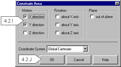
We are going to constrain the inside faces of the holes from translating in the
X and Y direction. Click on the check
boxes next to X direction and Y direction.
J. ![]() Click
OK. The symbols for the constraints will now appear on the inside hole faces
of the model. If the symbols disappear,
you may need to click on the Boundary Conditions
button to display them.
Click
OK. The symbols for the constraints will now appear on the inside hole faces
of the model. If the symbols disappear,
you may need to click on the Boundary Conditions
button to display them.
K. 
![]() Click
on the Constrain Area button
again. The Picker dialog will appear.
Click
on the Constrain Area button
again. The Picker dialog will appear.
L. Pick
the bottom face of the counterbored hole on both the upper and

lower attachment locations as shown. (Just the 2 holes shown)
M. 
Click OK on the Picker dialog. The Constrain
Area dialog will appear.
N.
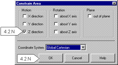
Constrain these areas in the Z direction only. Check on only the Z direction
check box. Click OK. The constraint symbols
will appear on these 2 faces.
Loads
To create loads
Choose the environment for which this Load applies.

Click the Add B.C. button.
Select Force to apply a force to the selected object(s).
![]()

With the cursor positioned on the Force button, hold down the left mouse
button. A fly-out toolbar appears. You can apply a force on a keypoint, a line,
or an area.
Click on the button representing the type force you want.
A picker appears. Select the keypoints, lines, or areas for applying the force. Click OK.
A Total Force on dialog box appears. Specify the value of the force in the required direction(s). This is the total force applied to all selected objects.
Select the coordinate system you want to apply if other than the Global Cartesian system. If you choose New Coordinate System, special conditions apply.
Click OK.

Select Moment to apply a moment to the selected Object(s)
![]()
With the cursor positioned on the Moment button, hold down the left mouse
button. A fly-out toolbar appears. You can apply a moment to a keypoint, a
line, or an area.
Click on the button representing type of entity you want to apply moment to.
A picker appears. Select the keypoints, lines, or areas to apply the moment to. Click OK.

A Total
Moment on dialog box appears. Specify the value of the moment in the
required direction(s).
Select the coordinate system you want to apply if other than the Global Cartesian system.
Click OK.

Select Displacement to set an
initial displacement on the selected object.
![]() With
the cursor positioned on the Displacement button, hold down the left mouse
button. A fly-out toolbar appears. You can displace a keypoint, a line, or an
area.
With
the cursor positioned on the Displacement button, hold down the left mouse
button. A fly-out toolbar appears. You can displace a keypoint, a line, or an
area.
Click on the button representing type of entity you want to apply displacement to.
 A picker appears. Select the keypoints,
lines, or areas to be displaced. Click OK.
A Total Displacement on dialog box
appears. Specify the displacement along the appropriate axes.
Select the coordinate system you want to apply if other than the Global Cartesian system.
Click OK.

Select Pressure to apply a pressure to either a line or area
![]()
With the cursor positioned on the Pressure
button, hold down the left mouse button. A fly-out toolbar appears. You can
apply pressure to a line or an area.
Click on the button representing type of entity you want to apply pressure to.
A picker appears. Select the lines or areas you are applying a pressure to and click OK.

A Pressure on dialog box appears. Enter the pressure value you want to apply.
Click OK.

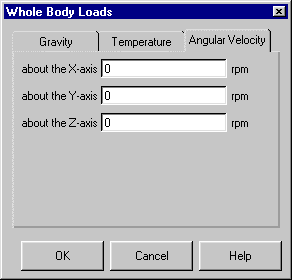
Select Body Load to apply a volumetric or field load. In the MTB, you can apply gravity, temperature, and angular velocity as body loads.
Click on the Body Load button.
A Whole Body Loads dialog box appears.
To apply gravity body loads, click the Gravity tab, enter the gravitational acceleration load values for the X, Y, and/or Z directions, then click OK.
To apply temperature body loads, click the Temperature tab and make choices depending on whether the temperature load is uniform or is a result of a thermal analysis.

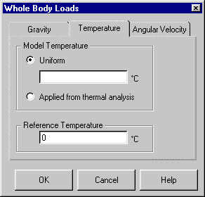
For a uniform temperature load, click the Uniform
radio button and enter the load temperature and the reference temperature, then
click OK.
To apply angular velocity body loads, click the Angular Velocity tab, enter the rotational speeds about the X, Y, and/or Z axes in revolutions per minute (RPM), then click OK.

 |
Select Model Symmetry, if you are a constructing a symmetric model, to define symmetry boundary conditions. These can be represented as an area on a 3-D model or a line on a 2-D (or 3-D shell) model.
Click the Model Symmetry button. A picker appears.
Select the line (for a 2-D model or 3-D shell model) or area (for a 3-D model) on which to define the symmetry boundary conditions.
Click OK.
Apply the loads to the model
A. ![]() Change
the view to better facilitate the loads application. Click on the Oblique View button.
Change
the view to better facilitate the loads application. Click on the Oblique View button.
B. 
![]() Click
and hold the left mouse button on Force
to get the fly out toolbar. Click on Area force. The Picker dialog will appear
Click
and hold the left mouse button on Force
to get the fly out toolbar. Click on Area force. The Picker dialog will appear
C.

Select the small area as shown (you may want to zoom up on the area) and click OK. The
Total Force on Area dialog will
appear.
D. Input
600 newtons for the force along the Y-axis and -1450 newtons for the Force along the Z-axis. Click on OK. The symbols for the

force will appear on the small area.
E. 
![]() Pick
the Area Force button again. The Picker will appear
Pick
the Area Force button again. The Picker will appear
F.
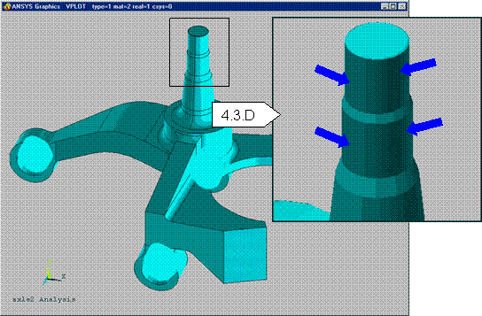
Pick the 4 areas on the axle as shown and select OK
G.
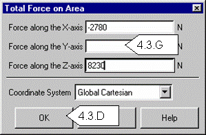
Input -2780 newtons for the Force
along the X-axis and 8230 newtons
for the Force along the Z-axis.
H. Click on OK. The symbols for the forces will appear on the axle.
Model Solution

Use the Solve tab to solve the
analysis. You can choose to solve now or solve later.
Solve Now
![]() To
solve now, select Solve Now from the
Solve Time drop down list box and
click the Solve Problem button.
To
solve now, select Solve Now from the
Solve Time drop down list box and
click the Solve Problem button.
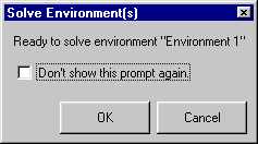
If you defined a single environment for a structural static or thermal
steady-state analysis, a Solve Environment(s) dialog box appears stating that
the environment is ready to be solved. Click the OK button to initiate the solution.
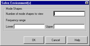
If you defined a single environment for a modal analysis, a Solve
Environment(s) dialog box appears. Enter the number of mode shapes you want to
view and the frequency range (if desired), then click OK to initiate the
solution.
If you defined multiple environments for a
structural static or thermal steady-state analysis, a Solve Environment(s) dialog box appears.
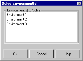
Choose the environment(s) you want to solve and click OK to initiate the solution(s).
When the solution is finished, the Mechanical Toolbar brings up the Results tab and automatically displays an appropriate plot (based on the discipline) and a text window that lists the environment(s), and summary information based on the discipline.
Solve Later
To solve later, follow these steps:
Select Solve Later... from the Solve Time drop down list box. A Solve Time dialog box appears.
Enter the date and time you want the solution to begin and click OK.
Click the Solve Problem button. A Solve Environment(s) dialog box appears whose content varies depending on the number of environments you want to solve and whether the problem involves a modal analysis .
Enter any required information in the Solve Environment(s) dialog box and click OK. A Solve Later Information dialog box appears which displays the solution start time that you entered, the working directory name and location where files will be stored, and a statement specifying that system specific processes must be running before using the solve later option.
If these systems are running, click OK to accept the name and location of the working directory, or specify another name and location for the working directory by clicking Browse..., choosing the name and directory location in the Solve Later Browse Working Directory dialog box, then clicking OK.
Solve the exercise
A. 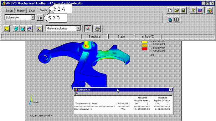
![]() Click
on the Solve tab on the MTB.
Click
on the Solve tab on the MTB.
B.  Click
on the Solve Problem button. The Solve
Environment(s) dialog will appear since there is only one environment.
C. Click OK to proceed with the solution. This may take a few minutes
D. When finished, a text window will appear showing that the solution successfully completed and will list the maximum displacement and stress. The graphics display will show the Von Mises Equivalent Stress plot. Note that the maximum stress value is well within the yield limit stress of steel.
Results
After completing a successful solution, it's now time to post process the model and take a look at the results. By default the MTB will select the Results tab after a successful solution.

To look at the results, click on the Results
tab
If you solved multiple load environments, you can view the results for each of them by:
Clicking on the Load Environment drop down list box.
Clicking on the environment for which you want to see results.
Results Item
You can view any of the following types of result information for a structural static analysis by clicking on the Results Item drop down list:
Equivalent stress - (Von Mises stress) a representation of any arbitrary stress state as a single positive stress value.
Displaced shape - physical displacement of the model.
Stress intensity - the difference between the maximum (1st) and minimum (3rd) principal stresses.
1st and 3rd principal stresses - The maximum and minimum principal stresses.
![]() Stress in the global X, Y, or Z direction
- individual stress components for each direction in the global Cartesian
system.
Stress in the global X, Y, or Z direction
- individual stress components for each direction in the global Cartesian
system.

After selecting the Results Item
click on Plot Results
Results Display

You can plot, query, animate, or list the result item shown in the Result Item
drop down list box.
![]() Click on the Plot Result button to plot the selected Results Item
Click on the Plot Result button to plot the selected Results Item
![]() To
query the results, click the Query
Result button. A picker appears. Hold the left mouse button down and drag
it over the area of interest. Result values appear both on the plot as well as
in the picker dialog.
To
query the results, click the Query
Result button. A picker appears. Hold the left mouse button down and drag
it over the area of interest. Result values appear both on the plot as well as
in the picker dialog.
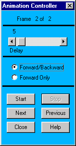

![]() To
animate the results, click the Animate
Result button. Click the black arrow to the right of the icon to specify
the number of frames to animate (default = 10 frames).
To
animate the results, click the Animate
Result button. Click the black arrow to the right of the icon to specify
the number of frames to animate (default = 10 frames).
An Animation Controller appears that allows you to start or stop the animation, play continuously or forward only, or apply delay.
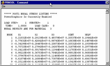
![]() Click
on the List Result button to see a
tabular listing of the results.
Click
on the List Result button to see a
tabular listing of the results.
Let's view the Result Items for this exercise
A. 
Change the Results Item to Displaced Shape
B.
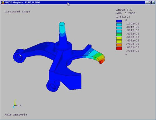
![]() Click
on the Plot Results button. The Displacement Shape plot will appear. The displacement are small in comparison to
the thickness of the model indicating good compliance with small displacement
theory
Click
on the Plot Results button. The Displacement Shape plot will appear. The displacement are small in comparison to
the thickness of the model indicating good compliance with small displacement
theory
C. Plot the other result items for kicks.
D. Return the plot to Equivalent Stress when you are done having fun.
E. 
![]() Animate
the results. Click on the arrow next to
the Animate button
Animate
the results. Click on the arrow next to
the Animate button
F.  Change
the number of frames to 8
G. ![]() Click
on the Animate button to start the
animation
Click
on the Animate button to start the
animation
H. Click on Close when you are satisfied.
I. Query the results. Click on the Query Results button. The Picker will appear.
J. Click on the Min and Max buttons on the picker to display a label indicating max and min stress.
K.
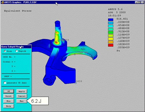
With your cursor click on some other areas to display the stress. If you click and hold the left mouse button
down and move it over the model the system will temporally display the stress
values.
![]() Reports
Reports

You can generate a report using a predefined format (template) or you can
generate a report using a template that you created. You can also view an
existing report. All reports are generated in standard HTML. You can forward
them electronically, post them on a web site, or print them.
The General Report format includes the following items:
Title page - name of analysis (taken from the Graphic Title entry in the Setup tab), name of analyst/designer (taken from the User Info tab [Toolbar Properties button within the main Setup tab]), date of report, links to Summary, Model Information, Analysis Information, and Results Information sections.
Summary - ANSYS plot of the original model, text summary including information on analysis type, environments, and results data.
Model Information - source of model file, ANSYS mesh plot, tabular details of the finite element model and material properties.
Analysis Information - ANSYS plot and tabular listings of loads and boundary conditions.
Results Information - ANSYS plots and tabular listings of results data.
To generate an HTML report using the predefined format, do the following:
Click on the Show Report button. The Report Options dialog appears.
Click on the Create a new report radio button.
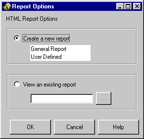
Click on the General Report option.
Click OK. The report is generated in the default HTML browser, and a directory named reportn is created (where n increments with each report generated) that includes the report's HTML file and all graphics files associated with the report.
To view an existing report, do the following:
Click the Show Report button. The Report Options dialog box appears.
Click the View an existing report radio button.
Type the directory path and file name of the HTML report file you want to view and click OK or use the Browse button to look through the directories and locate the report.
Create a Report
A. 
![]() Click
on the Show Report button
Click
on the Show Report button
B.
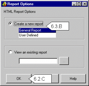
Toggle ON the Create a new report
options and click on General Report
C. Click OK. The report generation may take a few minutes. ANSYS will generate a professional looking report summarizing the model definition including element type, number of nodes and elements, applied loads, and constraints. All stresses, displacements and reaction force components will be plotted and summarized as well.
D. When complete, ANSYS will launch the report in your Internet browser. Take a few moments to review each section. This report can be customized and included in other documentation by cut and paste, or through hyperlinks.
E. For a sample HTML report, click here.
Conclusion:
The true intent of this exercise was to guide you through the Mechanical Toolbar and explain the various options that are available to you. The analysis of the axle showed that the part displayed no signs of yield under the given loading condition. Mesh refinements can be made in localized areas to determine more accurate stress values, but we will explore that in later exercises.

Additional Functions:
![]() New
Model:
New
Model:
This option allows you to clears the database stored in memory and start with a new one.
![]() Resume
Model:
Resume
Model:
Restores the database from the database file as it was at the last time that it was saved. This button is valid only for resuming database files that were generated using the Mechanical Toolbar. If you want to bring an ANSYS model into the Mechanical Toolbar, you need to use the Import Geometry button instead.
![]() Save
Model:
Save
Model:
Saves the current model to a database file.
A. ![]() Let's
save our work. Click on the Save button in the MTB.
Let's
save our work. Click on the Save button in the MTB.
Context Help:
Invokes your system's default Web browser and displays the table of contents for the Mechanical Toolbar's HTML-based help.
![]() Tour:
Tour:
Displays the Mechanical Toolbar's tour help. The tour provides an overview of the Mechanical Toolbar, its controls, and how to use it to perform an analysis.
![]() Fully
Functional ANSYS:
Fully
Functional ANSYS:
Switches to full ANSYS functionality. Note that only one environment may be brought over.
System Calculator:
![]() Invokes
the system calculator Use the Toolbar Properties dialog box to define the
system calculator.
Invokes
the system calculator Use the Toolbar Properties dialog box to define the
system calculator.
![]() System
Editor:
System
Editor:
Invokes the system editor (if one is available). Use the Toolbar Properties dialog box to define the system editor.
|