Bike Frame Analysis

This exercise will analyze a new, innovative mountain bike frame design under structural loads. The objective is to determine the maximum stresses in the frame due to the weight of a large rider for 3 different loading conditions. The model has already been sufficiently defeatured to facilitate building the finite element model. The exercise will use the no defeature/repair option during the Parasolid import. Shell elements will be used and a ½ symmetry model will be meshed using the Mechanical Toolbar (MTB). Symmetry boundary conditions and loads will also be applied in the MTB, along with the built-in properties for Titanium.

Important: Please Read the Following

This exercise contains the step by step instructions to complete the problem described above. All instructions to the exercise are denoted by Blue colored text.

This exercise also contains detailed information about the functions on Mechanical Toolbar. The information that is provided covers the required functions necessary to complete this exercise. Other functions will be covered in later exercises. The information should be read before proceeding with the instructions. The detailed information is denoted by the Black colored text.

Outline:

Launch ANSYS/Professional

Launch ANSYS using start menu.

Activate the Mechanical Toolbar.

Setup

Setting the Analysis Type.

Model

Model Import

Shell Properties

Viewing the Model

Defining Shell Or 2-D Solid Shapes

Assign Shape

Assigning Shell Properties to The Model

Assigning Other Shell Properties to The Model

Assign Material Properties To The Model

Meshing Using Smartsizing

Loads And Boundary Conditions

Applying Boundary Constraints To The Model

Create The Symmetry Boundary Constraints.

Renaming Environments

Copying Environments

Creating Loads For Combo Environment

Creating Loads For Standing Environment

Creating Loads For Sitting Environment

Save the Model

Solve Linear Elastic Solution

Solving With Multiple Environments

Linear Elastic Solution Results

Post Processing

Complete the following

Finding areas of maximum

Complete the following

Animate the Results

Create a Report

Review

Review Problem

Conclusion

Step-by-step Instructions:

Before beginning this problem, create a separate folder on your computer for this job and copy the bike parasolid file bike.xmt_txt to this folder.

If you do not have a parasolid translator, copy the file bike.db instead. When you reach section 3.1 (Model Import), select ANSYS (*db*) for type of file and import the bike.db file.

Launch ANSYS/Professional

Launch ANSYS using start menu.

A. Browse to select the working directory you just created for this job.

B. Change the Graphics device name to 3D

C. Enter bike for the Initial jobname. All ANSYS files created for this problem will have a filename of bike followed by a unique extension.

D. Change the Memory Requested for Total Workspace and for Database sizes for this job to be 256 and 64 respectively.

E. Click RUN to start the ANSYS GUI. 929u2018j

The following step is required only if you are not running ANSYS Professional.

The following step is required only if you are not running ANSYS Professional.

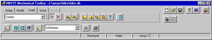
Activate the Mechanical Toolbar (MTB)

A. Click on MenuCtrls.

B.
Click on Mechanical Toolbar. The Mechanical Toolbar (MTB) will now appear and replace the Main Menu, Input Window, and the Toolbar.

Setup

Setting the Analysis Type. In the Mechanical Toolbar (MTB), let's set the basic analysis type options.

A. Set the Engineering Discipline to Structural.

B. Set the Analysis Type to Static.

C. Set the Unit System to m-kg-s-°C.

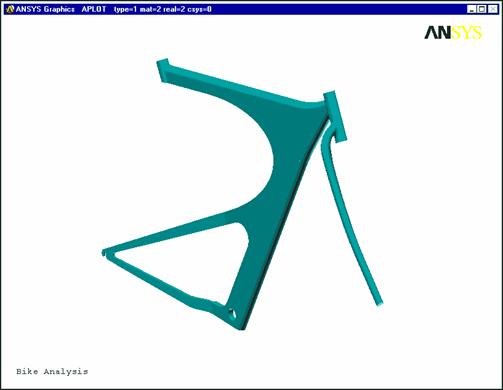
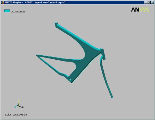
D. Type in Bike Analysis for the Graphic Title for the analysis.

E. This step is optional. Click on the Toolbar Properties button. The Toolbar Properties dialog will appear.

F.

Click on the User Info tab.

G. Enter your Name, Company, and Address.

H. Click OK when finished.

Model

Model Import: Under the Model tab, we import the geometry file, assign shell element thickness, material properties, and mesh the part.

A.
Click on the Model tab in the MTB.

B. Click on the Import geometry button to bring up the Model Import dialog.

C.

Change the Files of type: option to Parasolid.

D. Change the Look in: directory to the directory containing the bike parasolid (bike)

E. In the file list, highlight the file named bike.xmt_txt.

F. Click Open.

Note: If you do not have a parasolid translator, copy the file bike.db instead. When you reach section 3.1 (Model Import), select ANSYS (*db*) for type of file and import the bike.db file.

The Import Geometry - Select Import Method dialog will appear Select

Shell or 2-D Solid.

G. Leave the No model clean-up (faster) option set.

H.

Click OK. This may take a few seconds. Since you are importing a shell area (surface) model The Shell Properties dialog will appear. In this dialog you are asked to input the shell properties.

Shell Properties

When importing a Shell or 2-D Solid, the Shell Properties dialog box will next appear to allow you to define the default property name and thickness for the model. Input a name and the shell element thickness in this dialog.

A.

Input 1mm thick for the Name and .001 for the Thickness.

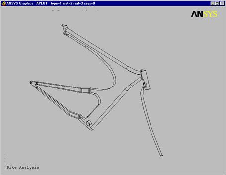
B. Click OK. ANSYS will now import the Parasolid file and draw the part in the graphics window.

C.
Use the dynamic viewing controls to inspect the model. Select the Pan-Zoom-Rotate button. If you are unfamiliar with the dynamic viewing controls, read the following pages.

Viewing the model

There are several buttons on the Mechanical Toolbar that allow you to manipulate graphic plots. These buttons and their functions include:

Plot: To access a fly-out toolbar of plotting options, do the following:

Position the cursor on the Plot button.

Press and hold the left mouse button until the fly-out toolbar appears.

The fly-out toolbar contains the following buttons: Keypoint Plot, Line Plot, Area Plot, Volume Plot, Node Plot, and Element Plot.

Release the left mouse button.

Position the cursor on the desired fly-out button and click.

Oblique View: Sets the view of the graphic window to oblique.

View: Sets the view of the graphic window. To access a fly-out toolbar:

Position the cursor on the View button.

Press and hold the left mouse button until the fly-out toolbar appears.

The fly-out toolbar contains the following View option buttons: Top View, Bottom View, Front View, Back View, Left View, Right View, Oblique View, Working Plane View, and Isometric View.

Pan-Zoom-Rotate: This option activates the Pan-Zoom-Rotate control, which allows you manipulate the model view by panning, zooming, or rotating the model. Note: This is a good option to leave on while working on the model.

To change the view, click on the desired view button (Top, Front, Iso, etc)

You can choose a Zoom method. Your options include: Zoom, Box Zoom, Win Zoom, and Back Up (UnZoom).

Pan/Zoom buttons: Pan up/down left/right using the arrows. Small dot zooms out and the large dot zooms in. The Rate slider located below the rotate buttons controls the amount of change in model size from zooming in or out.

The Rotate buttons allow you to define the axis of rotation. The rate slider that is below the rotate buttons controls the amount of rotation.

Dynamic Mode: This option allows you to use your mouse buttons to pan/zoom/rotate. When this is on, the left mouse button pans, the middle mouse button zooms, and the right mouse button rotates.

Lighting: This option allows you to control the light source location, intensity, and the reflectance of your model. When this option is ON the mouse buttons function as follows: Left Button: Move in X-direction to increase or decrease the reflectance of your model. Move in the Y-direction to change the intensity of the directional lights (there are two directional lights, one in front and one behind your model). Middle Button: Move in the X-direction to rotate the directional lights about the screen Z-axis. Move in the Y-direction to change the intensity of the ambient light. Right Button: Move in the X-direction to rotate the directional lights about the screen Y-axis. Move in the Y-direction to rotate the lights about the screen X-axis.

Fit: Automatically adjusts that amount of zoom in the active window so that your entire model can be seen within the window.

Reset: Removes any Pan-Zoom-Rotate changes in the active window. Your model will be displayed in its default orientation and sized to fit within the active widow.

Close: Dismisses the Pan-Zoom-Rotate dialog box.

Alternatives to using the Pan-Zoom-Rotate control

Pan - Hold down the CTRL key and press the left mouse button. Move the mouse left, right, up, or down to move the model in the desired direction.

Zoom - Hold down the CTRL key and press the middle mouse button. Move the mouse up to zoom in. Move the mouse down to zoom out. If you are using a two-button mouse, you may be able to mimic the action of a middle mouse button by holding down the SHIFT key and pressing the right mouse button.

Rotate about Z axis - Hold down the CTRL key and press the middle mouse button. Move the mouse left or right to rotate the model about the Z axis. If you are using a two-button mouse, you may be able to mimic the action of a middle mouse button by holding down the CTRL-SHIFT key and pressing the right mouse button.

Rotate about X or Y axis-Hold down the CTRL key and press the right mouse button. Move the mouse to rotate the model about the X (up/down) or Y (left/right) axis.

Redraw Model: Redraws (refreshes) the contents of the graphic window.

Render Model: This option allows you to set the render options for the model. The render options include material coloring, material texturing, thickness, translucency, wireframe, gray scale, and show edges.

Boundary Conditions: Toggles boundary condition symbols on and off.

Print Hardcopy: Prints a hardcopy of the graphic window contents.

A. Select the Pan-Zoom-Rotate button.

B. Thoroughly inspect the model by Panning, zooming, and rotating the model. Play with the light source option.

C. Return the view to Oblique when you are finished. Leave the Pan-Zoom-Rotate control open for the rest of the exercise

Defining Shell or 2-D Solid Shapes

To define element shapes for a model, click on the Default Shape drop down list and choose an element shape that you want to use.

All of the element shapes listed below are available in the Mechanical Toolbar. However, the choices that appear in the Default Shape drop down list box during a particular analysis will vary depending on the characteristics of the model that you imported.

Shell

Used to model thin structures in 3-D space. Can also be used for 2-D representations of such structures.

Solid

Used to model thick structures in 3-D space.

Plane Stress

Used to model thin planar structures in 2-D space.

Plane Strain

Used to model "infinitely long" structures having a constant cross-section in 2-D space.

Axisymmetric

Used to model solid structures with an axis of rotational symmetry in 2-D space.

Assign Shape

if you have more than one shape in the model, select an element shape from the Default Shape drop down list and assign the shape to entities in the model.

When you choose Shell in the Default Shape drop down list, the Shell Properties dialog box appears.

In the Name text entry box, type a unique name to identify this shell. It is useful to include the thickness of the shell in the name.

In the Thickness text entry box, type the thickness of this shell.

Click OK. The name of the defined shell shape will appear in the Default Shape drop down list.

You can view (but not change) the Name and Thickness properties of a shape by right-clicking in the Default Shape drop down list box and then selecting Properties.

A.
Create another shell property. Click on the Default Shape window and highlight Shell. The Shell Properties dialog will appear.

B. Input the name 2mm thick and .002 (meters) for the thickness.

C. Click OK.

Assign the 1mm thick shape property to the model.

A.
Click on the Default Shape window and pick the 1mm thick property

B. Click on the Assign Shape button. A dialog box for picking will appear.

C.

Click on the Pick All button. The system will select all areas and apply the 1mm thick properties to them. Notice that the model rendering has changed to plot the model thickness. The legend will indicate that all areas are 1mm thick.

Assign the 2mm thick shape property to the areas shown

A.
Click on the Render Model drop down list and pick Wireframe to better facilitate the next picking sequence.

B. Click on the Default Shape window and pick the 2mm thick property.

C. Click on the Assign Shape button. The picker will appear.

D. Refer to the diagram to the right. Zoom up on Area A

E. Pick the 3 highlighted areas shown below.

Tips for selecting areas: If you click and hold the left mouse button while dragging across the screen, each area to be selected will be highlighted. The area is not actually selected until you release the button. The hot spot for each area is the geometric center, which may not even lie on that area if it is a curved surface like the fillets. You can use the dynamic viewing controls to obtain a better orientation for selecting each area during the selection process. If you accidentally select a wrong area, click the right mouse button. The cursor will change from an upward pointing arrow to a downward pointing arrow indicating that you can now unpick items from the selection with the left mouse button. Click the right button again to toggle back to picking. When you have selected all the areas, click OK.

F. Select Fit on the Pan-Zoom-Rotate control dialog to see the whole bike.

G. Refer to the diagram. Zoom up on Area D

H.

Pick the 3 highlighted areas shown below. Fit the view when finished

I. Refer to the diagram. Zoom up on Area C

J.

Pick the 2 highlighted areas shown below. Fit the view when finished

K. Refer to the diagram. Zoom up on Area B

L. Change the picker option to Box

M.
Enclose the rear axle attachment with a selection box as shown below. Check the Count in the Picker dialog. You should have 24 picked areas

N. Select OK in the picker and then Fit the model. Notice the color coding between the 2 shell properties.

Assign Material Properties

A.
Now we want to assign the material properties to the entire model. Click on the Assign Material button. The Material for Assignment dialog will appear

B. ANSYS has built in properties for Aluminum, Steel and Titanium. Highlight Titanium in the list.

C. Click Continue. The picker will appear.

D. Click the Pick all button

E.

The model rendering will automatically change to Material Coloring and the legend will indicate that the entire part is Titanium.

Meshing: We will use the default SmartSize meshing to create a mesh on the part

A.
The slider bar in the MTB controls the SmartSize mesh density in various levels from very fine (left most setting) to very course (right most setting). Set the slider bar to the 6^th notch.

B. Click on the Mesh Model button to create the mesh.

C. The picker will appear asking you to select areas for meshing. Click on the Pick All button. ANSYS will mesh the model, which may take a few minutes. When meshing is complete, the mesh will briefly appear in the graphics window, and then disappear.

D. On the MTB, click and hold on the Plot button momentarily until the fly-out options appear.

E. Click on the far right fly-out button to Plot Elements. The model should look as shown below.

Loads and Boundary Conditions

Now that we have completed the model definition phase, it's time to apply the loads and boundary conditions. 3 different environments will be created with the same boundary conditions but different loads. The first load environment will be the entire weight of the rider on the seat. The second load environment will be the entire weight of the rider on the pedals and the third load environment will be the weight of the rider distributed on the seat, pedals, and handlebars.

Apply the boundary constraints to the model

A. 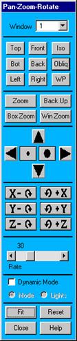Click on the Load tab in the MTB. Notice that the current environment is Environment 1.

B. Make sure the Add button is depressed.

C. Change the Render Model to Wireframe to aid in picking the correct areas.

D.

Change the display to an isometric view. Select ISO on the Pan-Zoom-Rotate dialog.

E. Click and hold the cursor on the Constraint button to get the fly-out
toolbar.

F. Click on Constrain Area. The Picker dialog will appear.

G.

Refer to the diagram below. Zoom up on area A

H. Pick the face on the rear wheel axle mount as shown. Fit the View

when finished.

I. Refer to the diagram. Zoom up on area B.

J.

Pick the end face on the front fork as shown. Fit the view when finished.

K.

Click on OK on the Picker. The Constrain area dialog will appear.

L.

Check on the constraints for Y direction, Z direction. These constraints will keep these areas from moving up/down and inward/outward but will allow movement forward/backward.

M. Click OK and then Fit the view. The constraint symbols will appear.

N.
If the constraint symbols did not appear, you may need to click on the Boundary Condition Button.

O.
Click on Area Constraint. The picker will appear.

P.

Refer to the diagram and then Zoom up on area C .

Q. Pick the 2 faces as shown.

R. Click OK on the picker dialog. The Constrain Area dialog will appear.

S. Check ON the motion constraint for X direction and click OFF the

motion constraints for Y direction and Z direction

T. Click OK.

U.

Fit the view. The constraint symbols will appear. This will hold the model from translating in the X-direction and prevent rigid body motion.

Create the Symmetry boundary conditions

A.
Change the view to a Right view. Click and hold on the View button to get the fly out toolbar.

B.

Pick the Right view option. The view should look as shown below.

C.
Click on the Model Symmetry button. The Picker will appear.

D.

Change the picker option to Box. Let's pick only the edges on the

symmetry plane. This may be a little tricky, so we will do this in 2 steps.

E. Create a selection box as shown. Make sure that the edges on the symmetry plane are enclosed.

F. Click OK. Little "S" symbols will appear indicating symmetry.

G.
If you were to inspect the model, you might find that a few extra lines might have been selected in the picking process. Therefore we need to delete these symmetry boundary conditions.

H. Click on Delete B.C.

I. Click on the Model Symmetry button. The Picker will appear

J. Change the picker option to Box.

K.
Create a selection box as shown below. Make sure that the edges on the symmetry plane are not enclosed.

L. Click OK on the Picker. Inspect the model. Make sure the "S" symbol is only on edges on the plane of symmetry

Rename Environment 1

A. Click in the Load Environment window to get the drop down list.

B.
Pick Rename Environment. You want to use descriptive names.

C.

The Rename Environment dialog will appear. Input Sitting in the To window. The sitting environment will simulate the riders weight (1424 N or 320 lbs) fully on the seat.

D. Click OK.

Make 2 copies of the current Boundary Condition so that we may use the same BC's for the different loading conditions.

A. Click in the Load Environment window to get the drop down list.

B.
Pick Copy Environment. The Copy Environment dialog will appear.

C. Input Standing in the To window. The standing environment will

simulate the rider's weight fully on the pedals.

D. Click OK. You now have a copy of the original boundary conditions.

E. Click in Load Environment window again to get the drop down list.

F.

Pick Copy Environment. The Copy Environment dialog will appear.

G.

Input Combo in the To window. The Combo environment will simulate the rider's weight distributed on the pedals, seat, and handlebars.

H. Click OK. You now have 2 copies of the original boundary condition.

I.
Turn OFF the boundary conditions display to aid in picking for the next step. Click on Boundary Conditions.

Create the Loads for the Combo environment.

A.
Make sure that Combo is the current environment and the Add button is depressed

B.

Change the view to the ISO View and the Model Render to Wireframe to better facilitate the load application.

C. Click and hold the left mouse button on Force to get the fly out toolbar.

D.

Click on Area force. The Picker dialog will appear.

E. Refer to the diagram above, and zoom up on Area A.

F.

Pick the highlighted area as shown. Fit the view when finished

G.

Refer to the diagram and zoom up on area B.

H. Pick the highlighted area as shown. Fit the view when finished.

I.

Refer to the diagram and zoom up on area C.

J. Select the highlighted area as shown.

K.

Click OK on the picker dialog. The Total Force on Area dialog will appear.

L. Input -712 (Newtons) for Force along the Y-axis. Since this is a symmetrical model the total load of 1424 N was divided in half.

M. Click OK to apply the load.

N. Fit the view to see the entire model

O. Click on the Boundary Conditions button to see the applied load

symbols.

P.
Click on the Boundary Conditions button again to hide the loads and BC's.

Create the Loads for the Standing environment.

A.
Click in the Load Environment window to get the drop down list.

B. Pick the Standing environment.

C. Click on Area force. The Picker dialog will appear.

D.

Refer to the diagram and zoom up on area B.

E. Pick the highlighted area as shown.

F. Click OK in the picker. The Total Force on Area dialog will appear.

G.

Input -712 (Newtons) for Force along the Y-axis.

H. Click OK. Fit the view.

I.
Click on the Boundary Conditions button to see the applied load.

J.

Click on the Boundary Conditions button again to hide the loads and BC's.

Create the Loads for the Sitting Environment.

A. Click in the Load Environment window to get the drop down list.

B. Pick the Sitting environment.

C.
Click on Area force. The Picker dialog will appear.

D. Refer to the diagram and zoom up on area A.

E. Pick the highlighted area as shown.

F. Click OK in the picker. The Total Force on Area dialog will appear.

G. Input -712 (Newtons) for Force along the Y-axis.

H. Click OK and then Fit the view.

I.
Click on the Boundary Conditions button to see the applied load.

Now is a good time to save the model.

A. Click on the Save button. The Save As dialog will appear.

B. Input the name Bike.

C. Select Save.

Solve Linear Elastic Solution:

We are ready to solve the model with the 3 environments

A.
Click on the Solve tab in the MTB.

B.

Click on the Solve Problem button. The Solve Environment(s) dialog will appear.

C. Select all 3 environments to solve.

D. Click OK. The solving process will take a few moments. Please be patient.

E.

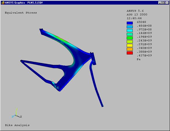
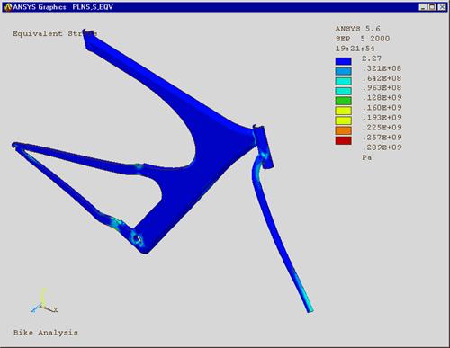
When finished, a text window will appear showing that the solution completed and will list the maximum displacement and stress. Close this box when finished reviewing. Also, a von Mises stress plot for the first environment will appear.

Linear Elastic Results:

We are ready for the post-processing phase.

A.
Click on the Results tab.

B. The von Mises stress should already be displayed. Use the pan/zoom/rotate function to review all portions of the model. Other components of stress as well as displacement can be plotted.

C. Change the Results Item to be shown from Equivalent Stress to 1st Principal Stress.

D.

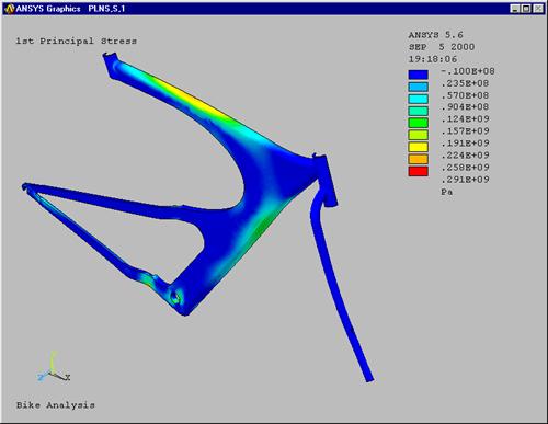
Click the Plot Results button.

E. You can also look at the different environments. Click on the Load Environment drop down list and pick Standing. The system will display
the Equivalent Stress plot for the Standing environment

.

Complete the following:

F. Determine which environment has the highest Equivalent stress.

G. Are there any stresses above the yield strength of Titanium (825Mpa)?

Find the area of maximum stress

A.
Plot the results for Equivalent stress for the Sitting environment. Set the Environment to Sitting.

B. Click on the Query button. The Query Subgrid Results dialog will appear.

C.

Click on Max. A label will appear on the model giving you the location of the Maximum Equivalent stress location.

D. Change the Results Item to Displaced Shape.

E.
Click on the Plot Results button. The Displacement Shape plot will appear. The displacements are small in comparison to the thickness of the model indicating good compliance with Shell element theory.

Complete the following:

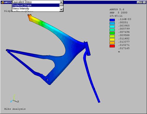F. Which loading environment produces the greatest displacement?

Animate the results.

A.

Click on the arrow next to the Animate button.

B.
Change the number of frames to 8.

C. Click on the Animate button to start the animation.

D. Click on Close when you are satisfied.

Create a Report

A.
Click on the Show Report button

B.

Toggle ON the Create a new report options and click on General Report

C. Click OK. The report generation may take a few minutes. ANSYS will generate a professional looking report summarizing the model definition including element type, number of nodes and elements, applied loads, and constraints. All stresses, displacements, and reaction force components will be plotted and summarized as well.

D. When complete, ANSYS will launch the report in your Internet browser. Take a few moments to review each section. This report can be customized and included in other documentation by cut and paste, or through hyperlinks.

Review

The following is a little review problem

A. Copy the Combo environment and name it Passenger

B. Add an additional Y axis load of -980 N at the handlebar location

C. Solve the model for only the Passenger environment

D. Review the results.

Conclusions:

The true intent of this exercise was to guide you through the Mechanical Toolbar for a different type of problem with some added complexity. You are now ready to proceed with more complex problems using the MTB and full ANSYS.

As for the bike, it seems clear that under the given loading the bike is more than capable of carrying the load and then some. The material thickness of the bike could be reduced to make it lighter.