Calibration
Definition. Calibrating is the process of tuning a model to fit detailed real data.
Calibrare = ajustarea parametrilor modelului pentru o mai mare apropiere de realitate)
or
Calibration - a test of the model with known input and output information that is used to adjust or estimate factors for which data are not available.
This is a multi-step, often iterative, process in which the model's processes are altered so that the model's predictions come to fit, with reasonable tolerance, a set of detailed real data. This approach is generally used for establishing the feasibility of the computational model; i.e., for showing that it is possible for the model to generate results that match the real data. This approach is more often used with emulation than with intellective models. Calibrating a model may require the researcher to both set and reset parameters and to alter the fundamental programming, procedures, algorithms, or rules in the computational model. Calibrating establishes, to an extent the validity of the internal workings of the model and its results (at least in a single case). The researcher may choose to halt calibration after achieving either a parameter or process level of validation.
To calibrate a model the researcher begins with the uncalibrated model. Then a trace of the model's predictions and the processes that generated them is generated. This information is then checked against real data. If the simulated predictions of the dependent variable(s) matches ? the real dependent variable the model is considered to be calibrated. Otherwise, first the parameters and then the processes are checked for accuracy. This check may involve going back and talking to experts at doing the task the model seeks to simulate or collecting new observational detail to fill in details or to check the accuracy of the original real data. Once both parameters and processes are accurate, if the model predictions are still not matching the real data, the modeler typically moves to adding additional lower level or auxiliary processes that were originally thought to be less important.
Problem: We have real values
r1, r2, ..., rn
and the simulation values
s1, s2, ..., sm
What do we mean by, or how do we decide if they "match"?
What if we do not have real values?
(Expert opinions)
Calibration occurs at two levels. At one level, the models predictions are compared against real data. This can be characterized as analysis of the dependent variable(s). At another level, the processes and parameters within the model are compared with data about the processes and parameters that produced the behavior of concern. This can be characterized as analysis of the independent (and control) variable(s). To calibrate a model it is important to have access to detailed data on one or more cases. Participant observation or other ethnographic data is often the best possible data for calibrating as typically only such data provides the level of detail needed by the modeler at both the process and outcome level. Calibrating models of subject matter experts typically requires interacting with an expert and discussing whether or not the model matches in its reasons and its results the behavior of the expert, and if not, why not.
In calibrating a model, the level of match required between the model and the real data depends in part on the research goals. The level of match also depends on the quality of the real data and the degree to which that data does not represent a pathologic or extreme data point. How should the cases for calibrating the computational model be chosen? The ideal is to use a set of cases that span the key categories across which the model is expected to operate. The next best option is to choose two to four cases that represent typical behavior and one to two that represent important extremes. The basic idea here is that by looking at both the typical and the extreme the boundaries on processes, parameters and outcomes can be set with some degree of confidence. In practice, however, the researcher who wishes to calibrate a model is often lucky to even have one case with sufficient detail.
That case, moreover, is often more a matter of opportunity than plan. Critics of calibration often argue that any model with sufficient parameters can always be adjusted so that some combination of parameters generates the observed data. Thus, the argument proceeds, calibration does not establish the validity of a model in a meaningful way. At one level, this criticism has some truth in it for some models. In particular, large multiparameter models often run the risk of having so many parameters that there is no guarantee that the model is doing anything more than curve fitting. However, for many computational models this criticism is less appropriate. In particular, for models where the process is represented not by parameterized equations but by rules, interactive processes, or a combination of procedures and heuristics there are often few if any parameters. There is no guarantee that a sufficiently large set of procedure and heuristics, that often interact in complex and non-linear ways, can be altered so that they will generate the observed data. For procedural models, calibration becomes a process of altering ''how things are done'' rather than ''how things are weighted.'' This distinction is critical as it separates process
matching from curve fitting.
References
Keith C. Clarke, Stacy Hoppen, and Leonard J. Gaydos
Methods And Techniques for Rigorous Calibration of a Cellular Automaton Model of Urban Growth
Abstract
Several lessons about the process of calibration were learned during
development of a self-modifying cellular automaton model to predict urban
growth. This model, part of a global change research project on human-induced
land transformations, was used to predict the spatial extent of urban growth
100 years into the future. The context of the prediction was to evaluate urban
environmental disturbances such as land use conversion, urban heat island
intensification, and greenhouse gas generation. Using data for the
Introduction
A cellular automaton urban growth model was developed and calibrated as part of the USGS Human-Induced Land Transformations project (HILT), part of a contribution to the U.S. Global Change Research Program (USGS, 1994). The study seeks to understand the urban transition from an historical and a multi-scale perspective sufficient to model and predict regional patterns of urbanization 100 years into the future (Kirtland et al., 1994).
The model provides regional predictions of urban extent to be used as a
basis for assessment of the ecological and climatic impacts of urban change and
estimation of the sustainable level of urbanization in a region. This paper
examines the initial calibration of the model using data from the
The Urban Transition Model
The urban model we developed is a scale-independent, cellular automaton model (Couclelis, 1985; Batty and Xie, 1994a; 1994b, White and Engelen, 1992). The growth rules are uniform throughout a gridded representation of geographic space and are applied on a cell-by-cell basis. All cells in the array are synchronously updated at the end of each time period. The basic principles of the growth rules, based on the Clarke wildfire model (Clarke et al., 1995), are general enough to describe any kind of organic expansion; they have been modified in this model to describe urban expansion. The growth rules are integral to the data set being used because they are defined in terms of the physical nature of the location under study, thus producing a scale-independent model.
The model was implemented as a computer program written in the C programming language. It operates as a set of nested loops: the outer control loop repeatedly executes each growth "history," retaining cumulative statistical data, while the inner loop executes the growth rules for a single "year." The starting point for urban growth is an input layer of "seed" cells, the urban extent for a particular year identified from historical maps, atlases, and other sources. The growth rules are applied on a cell-by-cell basis and the array is synchronously updated. The modified array forms the basis for urban expansion in each succeeding year. Potential cells for urbanization are selected at random and the growth rules evaluate the properties of the cell and its neighbors (e.g., whether or not they are already urban, what their topographic slope is, how close they are to a road). The decision to urbanize is based both on mechanistic growth rules as well as a set of weighted probabilities that encourage or inhibit growth. The model is described in detail in Clarke et al. (1996).
Five factors control the behavior of the system. These are: a diffusion factor, which determines the overall outward dispersiveness of the distribution; a breed coefficient, which specifies how likely a newly generated detached settlement is to begin its own growth cycle; a spread coefficient, which controls how much organic expansion occurs from existing settlements, a slope resistance factor, which influences the likelihood of settlement extending up steeper slopes; and a road gravity factor which attracts new settlements toward and along roads. These values, which affect the acceptance level of randomly drawn numbers, are set by the user for every model run.
Four types of growth are defined in the model: spontaneous, diffusive, organic, and road influenced growth. Spontaneous growth occurs when a randomly chosen cell falls nearby an already urbanized cell, simulating the influence urban areas have on their surroundings. Diffusive growth permits the urbanization of cells which are flat enough to be desirable locations for development, even if they do not lie near an already established urban area. Organic growth spreads outward from existing urban centers, representing the tendency of cities to expand. Road influenced growth encourages urbanized cells to develop along the transportation network replicating increased accessibility.
A second level of growth rules, termed self-modification, is prompted by an unusually high or low growth rate. The growth rate is the sum of the four different types of growth defined by the model for each model iteration or "year." The limits of "critical high" and "critical low" kick off an increase or decrease in three of the growth control parameters: diffusion, breed, and spread. The increase to the parameters is by a multiplier greater than one, "boom," imitating the tendency of an expanding system to grow ever more rapidly, while the decrease is by a multiplier less than one, "bust", causing growth to taper off as it does in a depressed or saturated system. However, to prevent uncontrolled exponential growth as the system increases in overall size, the multiplier applied to the factors is slightly decreased in every subsequent growth year.
Other effects of self-modification are an increase in the road gravity factor as the road network enlarges, prompting a wider band of urbanization around the roads, and a decrease in the slope resistance factor as the percentage of land available for development decreases, allowing expansion onto steeper slopes. Under self-modification the parameter values increase most rapidly in the beginning of the growth cycle when there are still many cells available to become urbanized, and decrease as urban density increases in the region and expansion levels off. Without self modification the model produces linear or exponential growth; self-modification was essential for modeling the typical S-curve growth rate of urban expansion.
Since the growth rules in this model are defined primarily by physical
factors, the
Four major types of data were compiled for this project: land cover, slope, transportation, and protected lands. Six raster image maps of urban extent for the years 1900, 1940, 1954, 1962, 1974, and 1990 were used. 1900 was the seed year, while the other years provided control data against which the model output was compared.
Calibration of the Model
The value of a model's predictions is only as good as the model's ability to be effectively calibrated. Since a model predicting future patterns can only be validated after the fact (when the authors will be unavailable) the validation step is not feasible. The calibration then is possible in only one way, by using the spatial and statistical properties of the past to "predict" the known present. In the HILT modeling effort, we have been using historical land use and satellite data from a variety of sources as calibration points for the model's behavior. At the very least, the model should be able to match the statistical patterns of past growth (within the constraints and limitations of the data) and to provide a probabilistic estimate of today's urban extent that matches reality. Even in the rich data environment in which we have worked, the time limitations of good calibration data are a severe challenge to predictive modeling. Often, a model outcome that performed perfectly statistically made little sense spatially. As a result, we have designed and undertaken a lengthy and computationally-intensive approach to model calibration that we believe to be rigorous.
The basic calibration approach was comparison of the model's output to an historical data set with respect to the key variable, urban areal extent. The Pearson product-moment correlation coefficient (r2) was used as a measure of fit between quantitative and spatial measures. The model's form of implementation evolved through two distinct calibration phases: a visual version which was most useful for broad parameter definition and debugging, and a faster, batch version of the model which was more efficient for generating the large quantity of runs necessary for calibration. The program computes and saves descriptive statistics in designated years 323i81d for comparison with the control years. The type of output has varied according to the needs of each step of the calibration.
The visual phase first established meaningful ranges of values for the growth parameters through an animation illustrating the impact of change in parameter values. Parameter values were increased by unit increments; each of the final outcomes became a single frame in the animation. Most parameters vary from 0 to 100, necessitating 101 separate runs per variable for the control variables. In each case, all other control variables were held constant at intermediate levels. This ascertained that each control parameter had a unique and controllable impact on the outcome, and it was noticed that some of the variables had clear saturation levels, beyond which increments had relatively little effect. Another benefit of this step was the informal verification that the form and rate of the model's growth was within reasonable bounds.
Two versions of the program with a full set of graphical user-interface tools evolved during this phase. The first was a prototype using the Silicon Graphics tools, which allowed easy animation and display of the resulting images (Figure 1). This version was used in generating animations from the data (Bell et al., 1994; Gaydos et al., 1995). The second version was an X Window System version. The XView toolset was used to create slider bars that allowed adjustment of the critical control parameters while the model was running and the ability to start and stop execution as necessary. This interactive environment provided a way of testing the control parameters' interaction with each other, and for debugging the self modification rules. In addition, a set of measures was explored to allow visual comparison between the actual and the predicted distributions. Symbols positioned on the animated maps showing the actual and predicted centers of gravity for the urban cells proved useful. Also used was the time-sequenced display of a circle with the same area as the predicted distribution drawn at the mean centers of the changing distribution. This allowed rapid visualization of structural changes in the spatial pattern. In addition, urban pixels were color-coded by which cellular automaton rule had invoked their transition.
![]() Three
statistical measures on the form of model growth were displayed on the screen
during this phase but were not thoroughly analyzed until the second,
graphics-free phase. These measures were the total area converted to urban use,
the number of pixels defined as edges, that is with non-urban cell neighbors,
which was felt a good measure of the rural-urban fringe nature of dispersed
distributions, and the number of separate spreading centers or clusters. The
number of spreading centers was computing using image processing algorithms, by
eroding the edges of the pattern without disconnecting clusters until each
cluster converged on a single pixel, and then counting the remaining pixels,
i.e. cluster centers.
Three
statistical measures on the form of model growth were displayed on the screen
during this phase but were not thoroughly analyzed until the second,
graphics-free phase. These measures were the total area converted to urban use,
the number of pixels defined as edges, that is with non-urban cell neighbors,
which was felt a good measure of the rural-urban fringe nature of dispersed
distributions, and the number of separate spreading centers or clusters. The
number of spreading centers was computing using image processing algorithms, by
eroding the edges of the pattern without disconnecting clusters until each
cluster converged on a single pixel, and then counting the remaining pixels,
i.e. cluster centers.
During the second phase of calibration, a CPU-optimized batch version of the model was produced, that was faster and more efficient at generating the vast quantity of runs necessary for calibration. Instead of displaying the three statistical measures on the screen (total area, number of edge pixels and number of clusters) the statistics were written into a set of log files for further analysis. An additional statistic became necessary during the non-visual phase, the Lee-Sallee shape index, a measurement of spatial fit between the model's growth and the known urban extent for the control years. This simple measure of shape was adjusted to describe distributions, and was computed by overlaying the observed and the predicted maps of urban extent, computing the union and the intersection of their total areas on a pixel by pixel basis, and then dividing the intersection by the union. For a perfect match, the Lee Sallee measure gives a value of 1.0, and for all others a smaller number, similar to an r-squared value. Inclusion of this statistic proved critical as there was no longer a means of identifying the best spatial match to historical growth now that the visual element was eliminated. These four values were aggregated into a combined score by adding the first three and multiplying by the shape index. The Lee-Sallee value is used as a multiplier because of its importance as a spatial measurement. A separate C program calculates the size, shape, number of clusters, and the Lee-Sallee statistic, as well as correlations between the predicted and observed data.
![]() The model requires initialization of five
growth parameters and four growth constants before operation, and these were
the nine variables adjusted during calibration. The calibration involved
finding the best combinations of the five growth parameters which regulate the
rate and nature of the types of growth: diffusion, spread, breed, slope
resistance, and road gravity. An additional task was definition of the four
growth constants which affect self-modification: critical high, critical low,
boom, and bust. While these four growth constants will always have the same
value at the end of a model run, the growth parameters may have different
values from the initial settings if the growth rate has exceeded the critical
high or critical low. The calibration strategy was to make minor changes in the
nine growth variables, and to compare the variations that resulted in the
combined r2 values. A semi-automated phase of the calibration began using shell
scripts to first hone in on the best range for each parameter, checking all
possible combinations of parameter settings in increments of five, then for a
narrower range of parameter values using unit increments.
The model requires initialization of five
growth parameters and four growth constants before operation, and these were
the nine variables adjusted during calibration. The calibration involved
finding the best combinations of the five growth parameters which regulate the
rate and nature of the types of growth: diffusion, spread, breed, slope
resistance, and road gravity. An additional task was definition of the four
growth constants which affect self-modification: critical high, critical low,
boom, and bust. While these four growth constants will always have the same
value at the end of a model run, the growth parameters may have different
values from the initial settings if the growth rate has exceeded the critical
high or critical low. The calibration strategy was to make minor changes in the
nine growth variables, and to compare the variations that resulted in the
combined r2 values. A semi-automated phase of the calibration began using shell
scripts to first hone in on the best range for each parameter, checking all
possible combinations of parameter settings in increments of five, then for a
narrower range of parameter values using unit increments.
From the unit increment runs, a sample of 160 different combinations of parameter settings was chosen, or about 10% of the possible number of combinations in the entire set of all possible runs. The statistics from these 160 combinations were examined in detail. To allow for the widely varying outcomes introduced by randomness in the growth process (each run used a different random number generator seed), each individual parameter combination was repeated 10 times, each run with 100 Monte Carlo iterations, creating a sample size of 1000 log files for each of the 160 combinations. The combined r2 value, described above, was used as the basis of comparison between these runs, the purpose being optimization of collective behavior. The statistical package SAS identified the parameter groups with the highest mean and the lowest standard deviation within the repetitions for the combined r2. Histograms of parameter values from the ten best combinations that emerged from this analysis were used to establish the ideal range of values for each parameter. A sensitivity analysis on the range established for each parameter was the final check using the mean and standard error of estimate for each initial parameter setting.
The other form of output from
the batch mode of calibration were
Evaluation of Calibration
Three sources of error can cause weak correlation during calibration: input error, model error, and parameter error (Debaeke, et al.). A change in the data source used to determine historical extent affected the r2 values edge and cluster. Creation of the historical urban extent layers were assembled from digitized paper maps for years before 1974, while in 1974 and 1990 remotely sensed images were used. The shapes on maps tend to have been generalized by the cartographer while satellite images have far more salt-and-pepper edges. Model error was weeded out early during establishment of parameters during the visual phase. Identical simulations were generated by forcing selection of a known random number seed. Parameter error occurs when the system variables are not independent, and of course this was the case as each parameter influenced more than one growth rule, as well as influencing each other during self-modification. Although a necessary aspect, self-modification introduced an additional level of complexity to the calibration process.
A major advantage of cellular modeling is that all input and output arrays are of a uniform size which permits easy quantitative comparisons between arrays through pixel counts and overlay and direct use of a GIS. Analysis of the output is facilitated as well because cells are of a uniform size and can be readily compared. Furthermore, multiple applications of the model from a variety of starting conditions allows the computation of Monte Carlo-style average aggregate output probabilities of any given cell being urbanized. We can then use the GIS to display, combine, and further analyze the model's predictive maps with other data as layers.
Predictions
Once the model had successfully replicated past urban expansion, it has
been used to project future scenarios of urban growth. Because these
predictions cannot be verified any time soon, any recommendations based on
these results must be understood in terms of probabilities. The predictions are
thought to be most valuable as a set of
Since the model output is a binary array that classifies each cell as urban or non-urban, it can be used to identify areas most at risk of urbanization, or as input to other models that need a layer defining urbanized areas as input, such as a climatology or a land use model. A second level of probability is implicit in these predictions: suffer time decay. As the model moves further into the future, the overall probabilities of predictions decline.
Conclusion
In this work, several important lessons were learned about the process of model calibration in addition to the success of the actual calibration effort itself. In terms of time, the calibration effort has taken as long as the period of model design and construction, and has overlapped productively with the debugging process. For example, only by preparing an animation of the final outcome of parameter range checking could the lack of impact of the parameter due to software bugs be detected, as during a single model run far too many interrelations between variables are taking place simultaneously to detect a lack of response.
The first lesson was that different phases of calibration were best served by radically different versions of the software. During the Model design stage, including initial experiments with small synthetic test data sets and the debugging of the model programs, an interactive graphic version of the model was essential. Literally thousands of graphic displays of model runs were observed while considering the impact of various control factors. We believe that there is no substitute for this "getting to know your data personally" phase. In many cases, the non-spatial nature of hidden or stylized model interface may mask not only errors in the model or data, but prevent the critical experimentation necessary for effective model design.
Secondly, we learned that it is valuable to build the tools necessary to
experiment with the model's full range of outcomes. In mathematics or physics,
the behavior of a function is first tested by examining behavior at the limits,
and no less is true of environmental models. In our case, the range of outcomes
came from parameter changes, computing outcomes over the full range of control
parameters, by
Thirdly, we learned that a rigorous mechanism for the evaluation of changing outcomes during calibration is required. The model had four constants and five variables to be assigned values. We used the initial conditions of the past to predict the present because we had key data slices that allowed the computation of measures of the goodness of fit. These measures had to be both statistical averages, and spatial descriptors. Addition of measures of the latter led to the ability to detect spurious outcomes, that although they generated correct numbers, made little sense geographically. We learned the zeroing in on an optimal configuration, in our case a set of initial conditions, required automated test procedures. For this we developed another version of the model and a selection of shell scripts that altered settings and recursively reran the programs, building a data base of outcomes that could be subjected to later statistical analysis. Analysis of these data, stored as log files, required links between the software, the GIS and the statistical package SAS.
Fourthly, we learned that animation is an important cartographic tool for all stages of the model's use, in showing variations in outcomes during debugging, in showing model runs during calibration, and as a tool for communicating the results of the model's predictions to modelers and non-modelers alike after completion of the model. This last lesson may be the most portable of all, that is that modelers are advised to make many spatial representations of their predictions, to use GIS-based cartographic and scientific visualization tools, and to use animation as a way of capturing non-modelers attention with your results.
The model we developed was somewhat special purpose. It was a scale independent cellular model, with some atypical properties such as the use of self-modification. Nevertheless, many of the lessons learned are generic to cellular models, and perhaps to all environmental models. Those working in environmental modeling should recognize the critical nature of calibration as a scientific process, as an opportunity to communicate the model's functions to a broader audience, as the solid ground upon which predictive work stands, and as an opportunity to seek out the limits, statistically and spatially, of a particular environmental model. Calibration should be an integral step in model design, should generate many of the tools for model use, and should build a rigorous scientific base for validation and predictive use of the model.
WATERSHED MODEL CALIBRATION AND VALIDATION:
THE HSPF EXPERIENCE
by
A. S. Donigian, Jr.
AQUA TERRA Consultants
Model calibration and validation are necessary and critical steps in any model application. For most all watershed models, calibration is an iterative procedure of parameter evaluation and refinement, as a result of comparing simulated and observed values of interest. Model validation is in reality an extension of the calibration process. Its purpose is to assure that the calibrated model properly assesses all the variables and conditions which can affect model results, and demonstrate the ability to predict field observations for periods separate from the calibration effort.
Model performance and calibration/validation are evaluated through qualitative and quantitative measures, involving both graphical comparisons and statistical tests. For flow simulations where continuous records are available, all these techniques should be employed, and the same comparisons should be performed, during both the calibration and validation phases. For water quality constituents, model performance is often based primarily on visual and graphical presentations as the frequency of observed data is often inadequate for accurate statistical measures.
Model performance criteria, sometimes referred to as calibration or validation criteria, have been contentious topics for more than 20 years. These issues have been recently thrust to the forefront in the environmental arena as a result of the need for, and use of modeling for exposure/risk assessments, TMDL determinations, and environmental assessments. Despite a lack of consensus on how they should be evaluated, in practice, environmental models are being applied, and their results are being used, for assessment and regulatory purposes. A 'weight of evidence' approach is most widely used in practice when models are examined and judged for acceptance for these purposes.
This paper explores the 'weight of evidence' approach and the current practice of watershed model calibration and validation based on more than 20 years experience with the U. S. EPA Hydrological Simulation Program - FORTRAN (HSPF). Example applications are described and model results are shown to demonstrate the graphical and statistical procedures used to assess model performance. In addition, quantitative criteria for various statistical measures are discussed as a basis for evaluating model results and documenting the model application efforts.
MODEL CALIBRATION AND VALIDATION
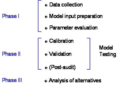
The modeling, or model application, process can be described as comprised of three phases, as shown in Figure 1 (Donigian and Rao, 1990). Phase I includes data collection, model input preparation, and parameter evaluation, i.e. all the steps needed to setup a model, characterize the watershed, and prepare for model executions. Phase II is the model testing phase which involves calibration, validation (or verification, both terms are used synonymously in this paper), and, when possible, post-audit. This is the phase in which the model is evaluated to assess whether it can reasonably represent the watershed behavior, for the purposes of the study. Phase III includes the ultimate use of the model, as a decision support tool for management and regulatory purposes.
Although specific application procedures for all watershed models differ due to the variations of the specific physical, chemical, and biological systems they each attempt to represent, they have many steps in common. The calibration and validation phase is especially critical since the outcome establishes how well the model represents the watershed, for the purpose of the study. Thus, this is the 'bottom-line' of the model application effort as it determines if the model results can be relied upon and used effectively for decision-making.
 Calibration
and validation have been defined by the American Society of Testing and
Materials, as follows (ASTM, 1984):
Calibration - a test of the model with known input and output information that is used to adjust or estimate factors for which data are not available.
Validation - comparison of model results with numerical data independently derived from experiments or observations of the environment.
|
Figure 1. The Modeling Process |
Model validation is in reality an extension of the calibration process. Its purpose is to assure that the calibrated model properly assesses all the variables and conditions which can affect model results. While there are several approaches to validating a model, perhaps the most effective procedure is to use only a portion of the available record of observed values for calibration; once the final parameter values are developed through calibration, simulation is performed for the remaining period of observed values and goodness-of-fit between recorded and simulated values is reassessed. This type of split-sample calibration/validation procedure is commonly used, and recommended, for many watershed modeling studies. Model credibility is based on the ability of a single set of parameters to represent the entire range of observed data. If a single parameter set can reasonably represent a wide range of events, then this is a form of validation.
In
practice, the model calibration/validation process can be viewed as a systematic
analysis of errors or differences between model predictions and field
observations. Figure 2 schematically
compares the model with the 'natural system', i.e. the watershed, and
identifies various sources 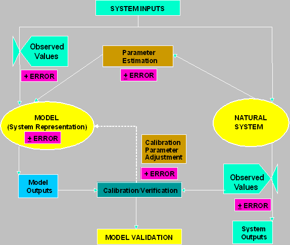
Figure 2. Model versus Natural System: Inputs, Outputs, and Errors
of potential errors to be investigated. These types of analysis requires evaluation of the accuracy and validity of the model input data, parameter values, model algorithms, calibration accuracy, and observed field data used in the calibration/validation. Clearly, the model user becomes a 'detective' in searching for the causes of the errors or differences, and potential remedies to improve the agreement and reduce the errors. A more complete discussion of these error sources is provided in Donigian and Rao (1990).
Model performance, i.e. the ability to reproduce field observations, and calibration/validation are most often evaluated through both qualitative and quantitative measures, involving both graphical comparisons and statistical tests. For flow simulations where continuous records are available, all these techniques will be employed, and the same comparisons will be performed, during both the calibration and validation phases. Comparisons of simulated and observed state variables will be performed for daily, monthly, and annual values, in addition to flow-frequency duration assessments. Statistical procedures include error statistics, correlation and model-fit efficiency coefficients, and goodness-of-fit tests.
For sediment, water quality, and biotic constituents, model performance will be based primarily on visual and graphical presentations as the frequency of observed data is often inadequate for accurate statistical measures. However, we will investigate alternative model performance assessment techniques, e.g. error statistics and correlation measures, consistent with the population of observed data available for model testing.
HSPF CALIBRATION AND VALIDATION PROCEDURES
Model application procedures for HSPF have been developed and described in the HSPF Application Guide (Donigian et al, 1984), in numerous watershed studies over the past 20 years (see HSPF Bibliography - Donigian, 2000), and most recently in HSPF applications to the Chesapeake Bay watershed (Donigian et al., 1994) and the Long Island Sound watersheds within the state of Connecticut (Love and Donigian, 2002). Model application procedures for HSPF include database development, watershed segmentation, and hydrology, sediment, and water quality calibration and validation.
As noted above, model calibration and validation are necessary and critical steps in any model application. For HSPF, calibration is an iterative procedure of parameter evaluation and refinement, as a result of comparing simulated and observed values of interest. It is required for parameters that cannot be deterministically, and uniquely, evaluated from topographic, climatic, edaphic, or physical/chemical characteristics of the watershed and compounds of interest. Fortunately, the large majority of HSPF parameters do not fall in this category. Calibration is based on several years of simulation (at least 3 to 5 years) in order to evaluate parameters under a variety of climatic, soil moisture, and water quality conditions. Calibration should result in parameter values that produce the best overall agreement between simulated and observed values throughout the calibration period.
Calibration includes the comparison of both monthly and annual values, and individual storm events, whenever sufficient data are available for these comparisons. All of these comparisons should be performed for a proper calibration of hydrology and water quality parameters. In addition, when a continuous observed record is available, such as for streamflow, simulated and observed values should be analyzed on a frequency basis and their resulting cumulative distributions (e.g. flow duration curves) compared to assess the model behavior and agreement over the full range of observations.
Calibration is a hierarchical process beginning with hydrology calibration of both runoff and streamflow, followed by sediment erosion and sediment transport calibration, and finally calibration of nonpoint source loading rates and water quality constituents When modeling land surface processes hydrologic calibration must precede sediment and water quality calibration since runoff is the transport mechanism by which nonpoint pollution occurs. Likewise, adjustments to the instream hydraulics simulation must be completed before instream sediment and water quality transport and processes are calibrated. Each of these steps are described briefly below.
Since
parameter evaluation is a key precursor to the calibration effort, a valuable
source of initial starting values for many of the key calibration parameters is
the recently-developed parameter database for HSPF, called HSPFParm (Donigian
et al., 1999). HSPFParm is an
interactive database (based on MS-Access) that includes calibrated parameter
values for up to 45 watershed water quality studies across the
Hydrologic Calibration
Hydrologic simulation combines the physical characteristics of the watershed and the observed meteorologic data series to produce the simulated hydrologic response. All watersheds have similar hydrologic components, but they are generally present in different combinations; thus different hydrologic responses occur on individual watersheds. HSPF simulates runoff from four components: surface runoff from impervious areas directly connected to the channel network, surface runoff from pervious areas, interflow from pervious areas, and groundwater flow. Since the historic streamflow is not divided into these four units, the relative relationship among these components must be inferred from the examination of many events over several years of continuous simulation.
A complete hydrologic calibration involves a successive examination of the following four characteristics of the watershed hydrology, in the following order: (1) annual water balance, (2) seasonal and monthly flow volumes, (3) baseflow, and (4) storm events. Simulated and observed values for each characteristic are examined and critical parameters are adjusted to improve or attain acceptable levels of agreement (discussed further below).
The annual water balance specifies the ultimate destination of incoming precipitation and is indicated as:
Precipitation - Actual Evapotranspiration - Deep Percolation
- Soil Moisture Storage = Runoff
HSPF requires input precipitation and potential evapotranspiration (PET), which effectively 'drive' the hydrology of the watershed; actual evapotranspiration is calculated by the model from the input potential and ambient soil moisture conditions. Thus, both inputs must be accurate and representative of the watershed conditions; it is often necessary to adjust the input data derived from neighboring stations that may be some distance away in order to reflect conditions on the watershed. HSPF allows the use of spatial adjustment factors that uniformly adjust the input data to watershed conditions, based on local isohyetal, evaporation, and climatic patterns. Fortunately, evaporation does not vary as greatly with distance, and use of evaporation data from distant stations (e.g. 50 to 100 miles) is common practice.
In addition to the input meteorologic data series, the critical HSPF parameters that affect components of the annual water balance include soil moisture storages, infiltration rates, vegetal evapotranspiration, and losses to deep groundwater recharge (see the BASINS web site, www.epa.gov/ost/basins/bsnsdocs/html, for information on HSPF parameters, including Tech Note #6 which provides parameter estimation guidance).
Thus, from the water balance equation, if precipitation is measured on the watershed, and if deep percolation to groundwater is small or negligible, actual evapotranspiration must be adjusted to cause a change in the long-term runoff component of the water balance. Changes in soil moisture storages (e.g. LZSN in HSPF) and vegetation characteristics affect the actual evapotranspiration by making more or less moisture available to evaporate or transpire. Both soil moisture and infiltration parameters also have a major impact on percolation and are important in obtaining an annual water balance. In addition, on extremely small watersheds (less than 200-500 acres) that contribute runoff only during and immediately following storm events, surface detention and near-surface soil moisture storages can also affect annual runoff volumes because of their impact on individual storm events (described below). Whenever there are losses to deep groundwater, such as recharge, or subsurface flow not measured at the flow gage, the recharge parameters are used to represent this loss from the annual water balance.
In the next step in hydrologic calibration, after an annual water balance is obtained, the seasonal or monthly distribution of runoff can be adjusted with use of the infiltration parameter. This seasonal distribution is accomplished by dividing the incoming moisture among surface runoff, interflow, upper zone soil moisture storage, and percolation to lower zone soil moisture and groundwater storage. Increasing infiltration will reduce immediate surface runoff (including interflow) and increase the groundwater component; decreasing will produce the opposite result.
The focus of the next stage in calibration is the baseflow component. This portion of the flow is often adjusted in conjunction with the seasonal/monthly flow calibration (previous step) since moving runoff volume between seasons often means transferring the surface runoff from storm events in wet seasons to low flow periods during dry seasons; by increasing the infiltration parameter runoff is delayed and occurs later in the year as an increased groundwater or baseflow. The shape of the groundwater recession, i.e. the change in baseflow discharge, is controlled by the groundwater recession rate which controls the rate of outflow from the groundwater storage. Using hydrograph separation techniques, these values are often calculated as the slope of the receding baseflow portion of the hydrograph; these initial values are then adjusted as needed through calibration.
In the final stage of hydrologic calibration, after an acceptable agreement has been attained for annual/monthly volumes and baseflow conditions, simulated hydrographs for selected storm events can be effectively altered by adjusting surface detention and interflow parameters. These parameters are used to adjust the shape of the hydrograph to better agree with observed values; both parameters are evaluated primarily from past experience and modeling studies, and then adjusted in calibration. Also, minor adjustments to the infiltration parameter can be used to improve simulated hydrographs. Examination of both daily and short time interval (e.g. hourly or 15-minute) flows may be included depending on the purpose of the study and the available data.
In addition to the above comparisons, the water balance components (input and simulated) should be reviewed for consistency with expected literature values for the study watershed. This effort involves displaying model results for individual land uses for the following water balance components:
Precipitation
Total Runoff (sum of following components)
. Overland flow
. Interflow
. Baseflow
Total Actual Evapotranspiration (ET) (sum of following components)
. Interception ET
. Upper zone ET
. Lower zone ET
. Baseflow ET
. Active groundwater ET
Deep Groundwater Recharge/Losses
Although observed values are not be available for each of the water balance components listed above, the average annual values must be consistent with expected values for the region, as impacted by the individual land use categories. This is a separate consistency, or reality, check with data independent of the modeling (except for precipitation) to insure that land use categories and overall water balance reflect local conditions.
In recent years, the hydrology calibration process has been facilitated with the aide of HSPEXP, an expert system for hydrologic calibration, specifically designed for use with HSPF, developed under contract for the U. S. Geological Survey (Lumb, McCammon, and Kittle, 1994). This package gives calibration advice, such as which model parameters to adjust and/or input to check, based on predetermined rules, and allows the user to interactively modify the HSPF Users Control Input (UCI) files, make model runs, examine statistics, and generate a variety of plots.
Snow Calibration
Since snow accumulation and melt is an important component of streamflow in many climates, accurate simulation of snow depths and melt processes is needed to successfully model the hydrologic behavior of the watershed. Snow calibration is actually part of the hydrologic calibration. It is usually performed during the initial phase of the hydrologic calibration since the snow simulation can impact not only winter runoff volumes, but also spring and early summer streamflow.
Simulation of snow accumulation and melt processes suffers from two main sources of user-controlled uncertainty: representative meteorologic input data and parameter estimation. The additional meteorologic time series data required for snow simulation (i.e. air temperature, solar radiation, wind, and dewpoint temperature) are not often available in the immediate vicinity of the watershed, and consequently must be estimated or extrapolated from the nearest available weather station. Snowmelt simulation is especially sensitive to the air temperature and solar radiation time series since these are the major driving forces for the energy balance melt calculations. Fortunately, additional nearby stations are available with air temperature data. The spatial adjustment factors, noted above, is used to adjust each of the required input meteorologic data to more closely represent conditions on the watershed; also, the model allows an internal correction for air temperature as a function of elevation, using a 'lapse' rate that specifies the change in temperature for any elevation difference between the watershed and the temperature gage.
In most applications the primary goal of the snow simulation will be to adequately represent the total volume and relative timing of snowmelt to produce reasonable soil moisture conditions in the spring and early summer so that subsequent rainfall events can be accurately simulated. Where observed snow depth (and water equivalent) measurements are available, comparisons with simulated values should be made. However, a tremendous variation in observed snow depth values can occur in a watershed, as a function of elevation, exposure, topography, etc. Thus a single observation point or location will not always be representative of the watershed average. See the BASINS Tech Note #6 for discussion and estimation of the snow parameters.
In many instances it is difficult to determine if problems in the snow simulation are due to the non-representative meteorologic data or inaccurate parameter values. Consequently the accuracy expectations and general objectives of snow calibration are not as rigorous as for the overall hydrologic calibration. Comparisons of simulated weekly and monthly runoff volumes with observed streamflow during snowmelt periods, and observed snow depth (and water equivalent) values are the primary procedures followed for snow calibration. Day-to-day variations and comparisons on shorter intervals (i.e. 2-hour, 4-hour, 6-hour, etc.) are usually not as important as representing the overall snowmelt volume and relative timing in the observed weekly or bi-weekly period.
Hydraulic Calibration
The major determinants of the routed flows simulated by the hydraulics section of HSPF, section HYDR are the hydrology results providing the inflows from the local drainage, inflows from any upstream reaches, and the physical data contained in the FTABLE, which is the stage-discharge function used for hydraulic routing in each stream reach. The FTABLE specifies values for surface area, reach volume, and discharge for a series of selected average depths of water in each reach. This information is part of the required model input and is obtained from cross-section data, channel characteristics (e.g. length, slope, roughness), and flow calculations. Since the FTABLE is an approximation of the stage-discharge-volume relationship for relatively long reaches, calibration of the values in the FTABLE is generally not needed. However, if flows and storage volumes at high flow conditions appear to be incorrect, some adjustments may be needed. Since HSPF cannot represent bi-directional flow, e.g. estuaries, linkage with hydrodynamic models is often needed to simulate tidal conditions and flow in rivers and streams with extremely flat slopes.
Sediment Erosion Calibration
Sediment calibration follows the hydrologic calibration and must precede water quality calibration. Calibration of the parameters involved in simulation of watershed sediment erosion is more uncertain than hydrologic calibration due to less experience with sediment simulation in different regions of the country. The process is analogous; the major sediment parameters are modified to increase agreement between simulated and recorded monthly sediment loss and storm event sediment removal. However, observed monthly sediment loss is often not available, and the sediment calibration parameters are not as distinctly separated between those that affect monthly sediment and those that control storm sediment loss. In fact, annual sediment losses are often the result of only a few major storms during the year.
Sediment loadings to the stream channel are estimated by land use category from literature data, local Extension Service sources, or procedures like the Universal Soil Loss Equation (USLE) (Wischmeier and Smith, 1972) and then adjusted for delivery to the stream with estimated sediment delivery ratios. Model parameters are then adjusted so that model calculated loadings are consistent with these estimated loading ranges. The loadings are further evaluated in conjunction with instream sediment transport calibration (discussed below) that extend to a point in the watershed where sediment concentration data is available. The objective is to represent the overall sediment behavior of the watershed, with knowledge of the morphological characteristics of the stream (i.e. aggrading or degrading behavior), using sediment loading rates that are consistent with available values and providing a reasonable match with instream sediment data. Recently a spreadsheet tool, TMDLUSLE, has been developed based on the USLE for estimating sediment loading rates as target values for calibration, and as a tool for sediment TMDL development; it is available from the U.S EPA website (www.epa.gov/ceampubl/tmdlusle.htm).
Instream Sediment Transport Calibration
Once the sediment loading rates are calibrated to provide the expected input to the stream channel, the sediment calibration then focuses on the channel processes of deposition, scour , and transport that determine both the total sediment load and the outflow sediment concentrations to be compared with observations. Although the sediment load from the land surface is calculated in HSPF as a total input, it must be divided into sand, silt, and clay fractions for simulation of instream processes. Each sediment size fraction is simulated separately, and storages of each size are maintained for both the water column (i.e. suspended sediment) and the bed.
In HSPF, the transport of the sand (non-cohesive) fraction is commonly calculated as a power function of the average velocity in the channel reach in each timestep. This transport capacity is compared to the available inflow and storage of sand particles; the bed is scoured if there is excess capacity to be satisfied, and sand is deposited if the transport capacity is less than the available sand in the channel reach. For the silt and clay (i.e. non-cohesive) fractions, shear stress calculations are performed by the hydraulics (HYDR) module and are compared to user-defined critical, or threshold, values for deposition and scour for each size. When the shear stress in each timestep is greater than the critical value for scour, the bed is scoured at a user-defined erodibility rate; when the shear stress is less than the critical deposition value, the silt or clay fraction deposits at a settling rate input by the user for each size. If the calculated shear stress falls between the critical scour and deposition values, the suspended material is transported through the reach. After all scour and/or deposition fluxes have been determined, the bed and water column storages are updated and outflow concentrations and fluxes are calculated for each timestep. These simulations are performed by the SEDTRN module in HSPF, complete details of which are provided in the HSPF User Manual (Bicknell et a., 1997; 2001).
In HSPF, sediment transport calibration involves numerous steps in determining model parameters and appropriate adjustments needed to insure a reasonable simulation of the sediment transport and behavior of the channel system. These steps are usually as follows:
Divide input sediment loads into appropriate size fractions
Run HSPF to calculate shear stress in each reach to estimate critical scour and deposition values
Estimate initial parameter values and storages for all reaches
Adjust scour, deposition and transport parameters to impose scour and deposition conditions at appropriate times, e.g. scour at high flows, deposition at low flows
Analyze sediment bed behavior and transport in each channel reach
Compare simulated and observed sediment concentrations, bed depths, and particle size distributions, where available
Repeat steps 1 through 5 as needed
Rarely is there sufficient observed local data to accurately calibrate all parameters for each stream reach. Consequently, model users focus the calibration on sites with observed data and review simulations in all parts of the watershed to insure that the model results are consistent with field observations, historical reports, and expected behavior from past experience. Ideally comprehensive datasets available for storm runoff should include both tributary and mainstem sampling sites. Observed storm concentrations of TSS should be compared with model results, and the sediment loading rates by land use category should be compared with the expected targets and ranges, as noted above.
The essence of watershed water quality calibration is to obtain acceptable agreement of observed and simulated concentrations (i.e. within defined criteria or targets), while maintaining the instream water quality parameters within physically realistic bounds, and the nonpoint loading rates within the expected ranges from the literature.
The following steps are usually performed at each of the calibration stations, following the hydrologic calibration and validation, and after the completion of input development for point source and atmospheric contributions:
Estimate all model parameters, including land use specific accumulation and depletion/removal rates, washoff rates, and subsurface concentrations
Superimpose the hydrology and tabulate, analyze, and compare simulated nonpoint loadings with expected range of nonpoint loadings from each land use and adjust loading parameters when necessary to improve agreement and consistency
Calibrate instream water temperature
Compare simulated and observed instream concentrations at each of the calibration stations
Analyze the results of comparisons in steps 3 and 4 to determine appropriate instream and/or nonpoint parameter adjustments, and repeat those steps as needed until calibration targets are achieved; Watershed loadings are adjusted when the instream simulated and observed concentrations are not in full agreement, and instream parameters have been adjusted throughout the range determined reasonable
Calibration procedures and parameters for simulation of nonpoint source pollutants will vary depending on whether constituents are modeled as sediment-associated or flow-associated. This refers to whether the loads are calculated as a function of sediment loadings or as a function of the overland flow rate. Due to their affinity for sediment, contaminants such metals, toxic organics, and phosphorous are usually modeled as sediment-associated, whereas BOD, nitrates, ammonia, and bacteria are often modeled as flow-associated.
Calibration of sediment-associated pollutants begins after a satisfactory calibration of sediment washoff has been completed. At this point, adjustments are performed in the contaminant potency factors, which are user-specified parameters for each contaminant. Potency factors are used primarily for highly sorptive contaminants that can be assumed to be transported with the sediment in the runoff. Generally, monthly and annual contaminant loss will not be available, so the potency factors will be adjusted by comparing simulated and recorded contaminant concentrations, or mass removal, for selected storm events. For nonpoint pollution, mass removal in terms of contaminant mass per unit time (e.g., gm/min) is often more indicative of the washoff and scour mechanisms than instantaneous observed contaminant concentrations.
Calibration procedures for simulation of contaminants associated with overland flow are focused on the adjustment of parameters relating to daily accumulation rates (lb/acre/day), accumulation limits (lb/acre), and washoff parameters (in/hr). As was the case for sediment-associated constituents, calibration is performed by comparing simulated and recorded contaminant concentrations, or mass removal, for selected storm events. In most cases, proper adjustment of corresponding parameters can be accomplished to provide a good representation of the washoff of flow-associated constituents. The HSPF Application Guide (Donigian et al., 1984) includes guidelines for calibration of these parameters, and the HSPFParm Database includes representative values for selected model applications for most conventional constituents.
In study areas where pollutant contributions are also associated with subsurface flows, contaminant concentration values are assigned for both interflow and active groundwater. The key parameters are simply the user- defined concentrations in interflow and groundwater/baseflow for each contaminant. HSPF includes the functionality to allow monthly values for all nonpoint loading parameters in order to better represent seasonal variations in the resulting loading rates.
In studies requiring detailed assessment of agricultural or forested runoff water quality for nutrients or pesticides, the mass balance soil module within HSPF, referred to as AGCHEM may need to be applied. Model users should consult the HSPF User Manual, the Application guide, and recent studies by Donigian et al (1998a, 1998b) that discuss application, input development, and calibration procedures.
Instream HSPF water quality calibration procedures are highly dependent on the specific constituents and processes represented, and in many ways, water quality calibration is equal parts art and science. As noted above, the goal is to obtain acceptable agreement of observed and simulated concentrations (i.e. within defined criteria or targets), while maintaining the instream water quality parameters within physically realistic bounds, and the nonpoint loading rates within the expected ranges from the literature. The specific model parameters to be adjusted depend on the model options selected and constituents being modeled, e.g. BOD decay rates, reaeration rates, settling rates, algal growth rates, temperature correction factors, coliform die-off rates, adsorption/desorption coefficients, etc. Part of the 'art' of water quality calibration, is assessing the interacting effects of modeled quantities, e.g. algal growth on nutrient uptake, and being able to analyze multiple timeseries plots jointly to determine needed parameter adjustments. The HSPF Application Guide and other model application references noted above are useful sources of information on calibration practices, along with model parameter compendiums published in the literature (e.g. Bowie et al., 1985).
MODEL PERFORMANCE CRITERIA
Model performance criteria, sometimes referred to as calibration or validation criteria, have been contentious topics for more than 20 years (see Thomann, 1980; Thomann, 1982; James and Burges, 1982; Donigian, 1982; ASTM, 1984). These issues have been recently thrust to the forefront in the environmental arena as a result of the need for, and use of modeling for exposure/risk assessments, TMDL determinations, and environmental assessments. Recently (September 1999), an EPA-sponsored workshop entitled "Quality Assurance of Environmental Models" convened in Seattle, WA to address the issues related to problems of model assessment and quality assurance, development of methods and techniques, assurance of models used in regulation, and research and practice on model assurance (see the following web site for details: https://www.nrcse.washington.edu/events/qaem/qaem.asp). This workshop spawned a flurry of web-based activity among a group of more than 50 recognized modeling professionals (both model developers and users) in various federal and state agencies, universities, and consulting firms that clearly confirms the current lack of consensus on this topic.
Although no consensus on model performance criteria is apparent from the past and recent model-related literature, a number of 'basic truths' are evident and are likely to be accepted by most modelers in modeling natural systems:
Models are approximations of reality; they can not precisely represent natural systems.
There is no single, accepted statistic or test that determines whether or not a model is validated
Both graphical comparisons and statistical tests are required in model calibration and validation.
Models cannot be expected to be more accurate than the errors (confidence intervals) in the input and observed data.
All of these 'basic truths' must be considered in the development of appropriate procedures for model performance and quality assurance of modeling efforts. Despite a lack of consensus on how they should be evaluated, in practice, environmental models are being applied, and their results are being used, for assessment and regulatory purposes. A 'weight of evidence' approach is most widely used and accepted when models are examined and judged for acceptance for these purposes. Simply put, the weight-of-evidence approach embodies the above 'truths', and demands that multiple model comparisons, both graphical and statistical, be demonstrated in order to assess model performance, while recognizing inherent errors and uncertainty in both the model, the input data, and the observations used to assess model acceptance.
Although all watersheds, and other environmental systems, models will utilize different types of graphical and statistical procedures, they will generally include some of the following:
Graphical Comparisons:
Timeseries plots of observed and simulated values for fluxes (e.g. flow) or state variables (e.g. stage, sediment concentration, biomass concentration)
Observed vs. simulated scatter plots, with a 45o linear regression line displayed, for fluxes or state variables
Cumulative frequency distributions of observed and simulated fluxes or state variable (e.g. flow duration curves)
Statistical Tests:
Error statistics, e.g. mean error, absolute mean error, relative error, relative bias, standard error of estimate, etc.
Correlation tests, e.g. linear correlation coefficient, coefficient of model-fit efficiency, etc.
Cumulative Distribution tests, e.g. Kolmogorov-Smirnov (KS) test
These comparisons and statistical tests are fully documented in a number of comprehensive references on applications of statistical procedures for biological assessment (Zar, 1999), hydrologic modeling (McCuen and Snyder, 1986), and environmental engineering (Berthouex and Brown, 1994).
Time series plots are generally evaluated visually as to the agreement, or lack thereof, between the simulated and observed values. Scatter plots usually include calculation of a correlation coefficient, along with the slope and intercept of the linear regression line; thus the graphical and statistical assessments are combined. For comparing observed and simulated cumulative frequency distributions (e.g. flow duration curves), the KS test can be used to assess whether the two distributions are different at a selected significance level. Unfortunately, the reliability of the KS test is a direct function of the population of the observed data values that define the observed cumulative distribution. Except for flow comparisons at the major USGS gage sites, there is unlikely to be sufficient observed data (i.e. more than 50 data values per location and constituent) to perform this test reliably for most water quality and biotic constituents. Moreover, the KS test is often quite easy to 'pass', and a visual assessment of the agreement between observed and simulated flow duration curves, over the entire range of high to low flows, may be adequate and even more demanding in many situations
In recognition of the inherent variability in natural systems and unavoidable errors in field observations, the USGS provides the following characterization of the accuracy of its streamflow records in all its surface water data reports (e.g. Socolow et al., 1997):
Excellent Rating 95 % of daily discharges are within 5 % of the true value
Good Rating 95 % of daily discharges are within 10 % of the true value
Fair Rating 95 % of daily discharges are within 15 % of the true value
Records that do not meet these criteria are rated as 'poor'. Clearly, model results for flow simulations that are within these accuracy tolerances can be considered acceptable calibration and validation results, since these levels of uncertainty are inherent in the observed data.
Table 1 lists general calibration/validation tolerances or targets that have been provided to model users as part of HSPF training workshops over the past 10 years (e.g. Donigian, 2000). The values in the table attempt to provide some general guidance, in terms of the percent mean errors or differences between simulated and observed values, so that users can gage what level of agreement or accuracy (i.e. very good, good, fair) may be expected from the model application.
|
Table 1 General Calibration/Validation Targets or Tolerances for HSPF Applications (Donigian, 2000) |
|
% Difference Between Simulated and Recorded Values |
|||
|
Very Good |
Good |
Fair |
|
|
Hydrology/Flow |
< 10 | ||
|
Sediment |
< 20 |
|
|
|
Water Temperature |
< 7 | ||
|
Water Quality/Nutrients |
< 15 | ||
|
Pesticides/Toxics |
< 20 | ||
CAVEATS: Relevant to monthly and annual values; storm peaks may differ more
Quality and detail of input and calibration data
Purpose of model application
Availability of alternative assessment procedures
Resource availability (i.e. time, money, personnel)
 The caveats at the bottom of the
table indicate that the tolerance ranges should be applied to mean values, and that individual events
or observations may show larger differences, and still be acceptable. In addition, the level of agreement to be
expected depends on many site and application-specific conditions, including
the data quality, purpose of the study, available resources, and available
alternative assessment procedures that could meet the study objectives.
|
Figure 3. R and R2 |
Figure 3 provides value ranges for both correlation coefficients (R) and coefficient of determination (R2) for assessing model performance for both daily and monthly flows. The figure shows the range of values that may be appropriate for judging how well the model is performing based on the daily and monthly simulation results. As shown, the ranges for daily values are lower to reflect the difficulties in exactly duplicating the timing of flows, given the uncertainties in the timing of model inputs, mainly precipitation.
Given the uncertain state-of-the-art in model performance criteria, the inherent errors in input and observed data, and the approximate nature of model formulations, absolute criteria for watershed model acceptance or rejection are not generally considered appropriate by most modeling professionals. And yet, most decision makers want definitive answers to the questions - 'How accurate is the model ?', 'Is the model good enough for this evaluation ?', 'How uncertain or reliable are the model predictions ?'. Consequently, we propose that targets or tolerance ranges, such as those shown above, be defined as general targets or goals for model calibration and validation for the corresponding modeled quantities. These tolerances should be applied to comparisons of simulated and observed mean flows, stage, concentrations, and other state variables of concern in the specific study effort, with larger deviations expected for individual sample points in both space and time. The values shown above have been derived primarily from HSPF experience and selected past efforts on model performance criteria; however, they do reflect common tolerances accepted by many modeling professionals.
EXAMPLE HSPF CALIBRATION/VALIDATION COMPARISONS
This
section presents results from recent HSPF applications, (1) to the State of
The
The
Connecticut Watershed Model (CTWM), based on HSPF, was developed to evaluate
nutrient sources and loadings within each of six nutrient management zones that
lie primarily within the state of
The hydrologic calibration for the Test Watersheds and the
Calibration
of the CTWM was a cyclical process of making parameter changes, running the
model and producing the aforementioned comparisons of simulated and observed
values, and interpreting the results. This process was greatly facilitated with the use of HSPEXP, an expert
system for hydrologic calibration, specifically designed for use with HSPF,
developed under contract for the USGS (Lumb, McCammon, and Kittle, 1994). This package gives calibration advice, such
as which model parameters to adjust and/or input to check, based on
predetermined rules, and allows the user to interactively modify the HSPF Users
Control Input (UCI) files, make model runs, examine statistics, and generate a
variety of plots. The postprocessing
capabilities of GenScn (e.g., listings, plots, statistics, etc.) were also used
extensively during the 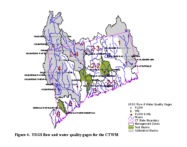
calibration/validation effort.
The hydrology calibration focused primarily on the monthly agreement of simulated and observed values as opposed to individual storm events, due to the greater sensitivity of LIS to long-term versus short-term nutrient loads (HydroQual, 1996).
The time period of the water quality calibration coincided with the hydrology calibration period, i.e. 1991-95. However, sufficient water quality data to support a validation were not available; the primary limitation being the lack of adequate point source data for the earlier period. In addition, both resource and data limitations precluded modeling sediment erosion and instream sediment transport and deposition processes, and their impacts on water quality. The calibration followed the steps discussed above for nonpoint and water quality calibration. The results presented here are a summary of the complete modeling results presented in the Final Project report with Appendices (AQUA TERRA Consultants and HydroQual, 2001).
Table 2 shows the mean annual runoff, simulated and observed, along with correlation daily and monthly coefficients for the six primary calibration sites. The CTWM hydrology results consistently show a good to very good agreement based on annual and monthly comparisons, defined by the calibration/validation targets discussed above. The monthly correlation coefficients are consistently greater than 0.9, and the daily values are greater than 0.8. The annual volumes are usually within the 10% target for a very good agreement, and always within the 15% target for a good agreement.
|
Table 2 Summary of CTWM hydrologic calibration/validation - annual flow and correlation coefficients |
|||||||||
|
Calibration Period (1991-1995) |
Validation Period (1986-1990) |
||||||||
|
Station Name |
Station Number |
Mean Observed Annual Flow (inches) |
Mean Simulated Annual Flow (inches) |
R Average Daily |
R Average Monthly |
Mean Observed Annual Flow (inches) |
Mean Simulated Annual Flow (inches) |
R Average Daily |
R Average Monthly |
|
Test Watershed Gages | |||||||||
|
Salmon River nr
| |||||||||
|
| |||||||||
|
| |||||||||
|
Major Basin Gages | |||||||||
|
| |||||||||
|
| |||||||||
|
| |||||||||
Figures 5 and 6 present graphical comparisons of
simulated and observed daily flows for the
Figure 5. Observed and Simulated Daily Flow for
the
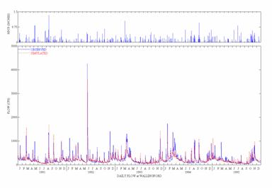
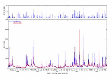 (Top curves are Daily
Precipitation)
![]()
Figure 6. Observed
and Simulated Daily Flow for the
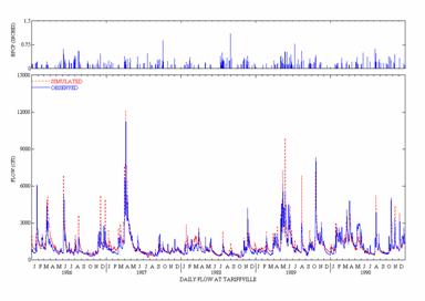
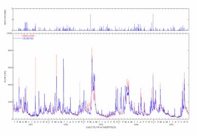 (Top curves are Daily Precipitation)
![]()
![]()
![]()
Figure 7. Observed and Simulated Daily Flow Duration
Curves for the
![]()
![]()
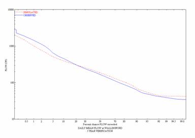
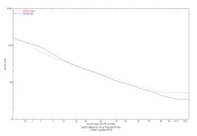
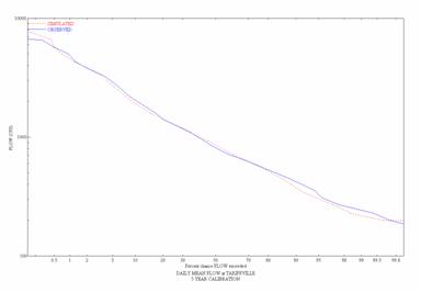
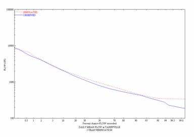 Figure
8. Observed and Simulated Daily Flow
Duration Curves for the
![]()
![]()
Figure 9. Scatterplots
of Observed and Simulated Daily and Monthly Flow for the
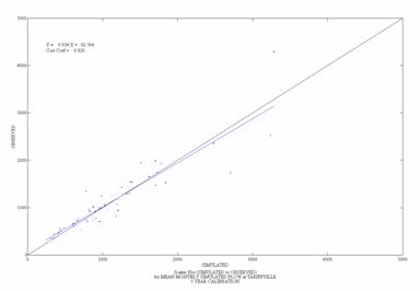
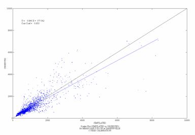 Daily Monthly
![]()
Figure 10. Scatterplots
of Observed and Simulated Daily and Monthly Flow for the
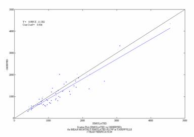
 Daily Monthly
![]()
Based on the general 'weight-of-evidence', involving both graphical and statistical tests, the hydrology component of the CTWM was confirmed to be both calibrated and validated, and provides a sound basis for the water quality and loading purposes of this study.
Water Quality Results
As noted above, the essence of watershed
water quality calibration is to obtain acceptable agreement of observed and
simulated concentrations (i.e. within defined criteria or targets), while
maintaining the instream water quality parameters within physically realistic
bounds, and the nonpoint loading rates within the expected ranges from the
literature. The nonpoint loading rates,
sometimes referred to as 'export coefficients' are highly variable, with value
ranges sometimes up to an order of magnitude, depending on local and site
conditions of soils, slopes, topography, climate, etc. Although a number of studies on export
coefficients have been done for
Frink's Export Coefficients (lb/ac/yr):
Total Nitrogen Total Phosphorus
Urban 12.0 " 1.5 "
Agriculture 6.8 " 0.5 "
Forest 2.1 " 0.1 "
The above loading rates were used for general guidance, to supplement our past experience, in evaluating the CTWM loading rates and imposing relative magnitudes by land use type. No attempt was made to specifically calibrate the CTWM loading rates to duplicate the export coefficients noted above. The overall calculated mean annual loading rates and ranges for Total N and Total P for 1991-95, are summarized as follows:
CTWM Loading Rates (lb/ac/yr)
Mean (range)
Total Nitrogen Total Phosphorus
Urban - pervious 8.5 (5.6 - 15.7) 0.26 (0.20 - 0.41)
Urban - impervious 4.9 (3.7 - 6.6) 0.32 (0.18 - 0.36)
Agriculture 5.9 (3.4 - 11.6) 0.30 (0.23 - 0.44)
Forest 2.4 (1.4 - 4.3) 0.04 (0.03 - 0.08)
Wetlands 2.2 (1.4 - 3.5) 0.03 (0.02 - 0.05)
Considering the purposes of the study, and the assumptions in the model development (e.g. sediment not simulated), these loading rates were judged to be consistent with Frink's values and the general literature, and thus acceptable for the modeling effort (see Final Report for details and breakdown of TN and TP into components).
Tables 3 and 4 display the mean simulated and observed concentrations for the five-year period for all of the water quality stations where calibration was performed. The comparison of mean concentrations, and the ratios of simulated to observed values, demonstrate that simulated values are generally within 20% of observed, i.e. the ratios are mostly between 0.8 and 1.2, and often between 0.9 and 1.1. The biggest differences are for the phosphorus compounds, where the ratios range from 0.91 to 1.9. Considering all the sites (Table 4), the mean value for the ratios for DO, TOC and nitrogen forms are within a range of 0.89 to 0.99, while the phosphorus ratios are 1.33 to 1.40. Comparing these ratios to the proposed calibration targets indicates a 'very good' calibration of nitrogen, and a borderline 'fair' calibration of phosphorus.
|
Table 3 Average Annual Concentrations (mg/L) for the Calibration Period (1991-1995) |
||||||||||||||||||
|
Salmon River nr
|
|
|
|
|
|
|||||||||||||
|
Constituent |
Observed |
Simulated |
Ratio * (sample size) |
Observed |
Simulated |
Ratio * (sample size) |
Observed |
Simulated |
Ratio * (sample size) |
Observed |
Simulated |
Ratio * (sample size) |
Observed |
Simulated |
Ratio * (sample size) |
Observed |
Simulated |
Ratio * (sample size) |
|
Dissolved Oxygen | ||||||||||||||||||
|
Ammonia as N | ||||||||||||||||||
|
Nitrite-Nitrate as N | ||||||||||||||||||
|
Organic Nitrogen |
| |||||||||||||||||
|
Total Nitrogen | ||||||||||||||||||
|
Orthophosphate as P | ||||||||||||||||||
|
Organic Phosphorus | ||||||||||||||||||
|
Total Phosphorus | ||||||||||||||||||
|
Total Organic Carbon | ||||||||||||||||||
Ratios calculated from Simulated and Observed concentrations prior to rounding
|
Table 4 Average and |
||
|
Constituent |
Average |
Range |
|
Dissolved Oxygen | ||
|
Ammonia as N | ||
|
Nitrite-Nitrate as N | ||
|
Organic Nitrogen | ||
|
Total Nitrogen | ||
|
Orthophosphate as P | ||
|
Organic Phosphorus | ||
|
Total Phosphorus | ||
|
Total Organic Carbon | ||
Figures 11 and 12 present typical graphical
comparisons made for simulated and observed water quality constituents. Figure 11 presents a comparison of simulated
and observed total phosphorus for the
Figure 11 Observed and Simulated Daily Total Phosphorus
Concentrations for the
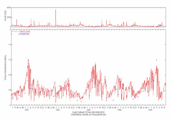
Figure 12 Observed and Simulated Daily Total Nitrogen
Concentrations for the
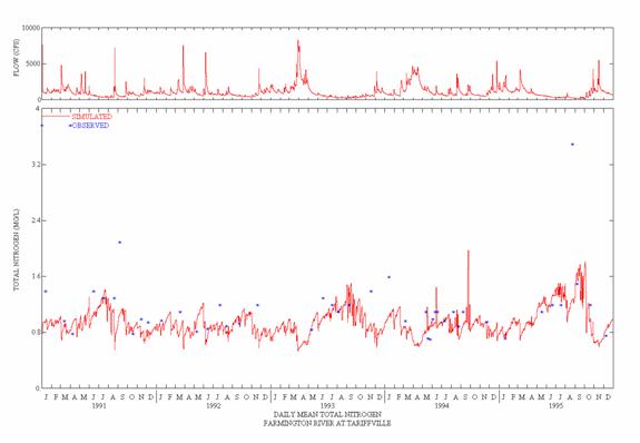
Based on the general 'weight-of-evidence' of the hydrology and water quality simulation results, including the CTWM loading rates, the mean concentrations and ratios, and the timeseries comparisons of observed and simulated values, the CTWM was determined to be an acceptable representation of the Connecticut watersheds providing loadings to LIS. This evidence indicates that the predicted nitrogen and carbon loadings are a 'very good' representation of the observed data, based on the established calibration targets, and that the phosphorus loadings are a 'fair' representation. Clearly improvements can be made to better represent these loadings, especially for phosphorus, but the CTWM in its current form is a sound tool for examining loadings to LIS and providing the basis for developing and analyzing alternative watershed scenarios designed to improve the water quality of LIS.
Unnamed
HSPF is currently being applied to
an almost 300 sq. mi. watershed in the
|
Table 5 |
||||
|
Unnamed Watershed |
||||
|
Precipitation |
Simulated Flow |
Observed Flow |
Percent Error |
|
|
Total | ||||
|
Average | ||||
Table 6 shows the statistical
output available from HSPEXP for both the 'Watershed Outlet' and an 'Upstream
Tributary' of about 60 sq. mi., while Table 7 shows a variety of statistics for
both daily and monthly comparisons at the watershed outlet. The storm statistics in Table 6 are based
on a selection of 31 events throughout
the 10-year period, distributed to help evaluate seasonal differences. The correlation statistics in Table 7
indicate a 'good' calibration for daily values,
|
Table 6 |
|||||
|
Upstream Tributary |
Watershed Outlet |
||||
|
Simulated |
Observed |
Simulated |
Observed |
||
|
Average runoff, in inches | |||||
|
Total of highest 10% flows, in inches | |||||
|
Total of lowest 50% flows, in inches | |||||
|
Evapotranspiration, in inches | |||||
|
Total storm volume, in inches2 | |||||
|
Average of storm peaks, in cfs2 | |||||
|
Calculated |
Criteria |
Calculated |
Criteria |
||
|
Error in total volume, % | |||||
|
Error in 10% highest flows, % | |||||
|
Error in 50% lowest flows, % | |||||
|
Error in storm peaks, % | |||||
1 - PET (estimated by multiplying observed pan evaporation data by 0.73)
2 - Based on 31 storms occurring between 1990 and 1999
|
Table 7 |
|||||
|
Unnamed Watershed |
|||||
|
Daily |
Monthly |
||||
|
Simulated |
Observed |
Simulated |
Observed |
||
|
Count | |||||
|
Mean, cfs | |||||
|
Geometric Mean, cfs | |||||
|
Correlation Coefficient (R) | |||||
|
Coefficient of Determination (R2) | |||||
|
Mean Error, cfs | |||||
|
Mean Absolute Error, cfs | |||||
|
RMS Error, cfs | |||||
|
Model Fit Efficiency (1.0 is perfect) | |||||
and a 'very good' calibration of monthly flows, when compared to the value ranges in Figure 3.
Table 8 shows the mean monthly observed and simulated runoff, along with their differences (or residuals) and '% error', as another assessment of the seasonal representation of the model; Figure 13 graphically shows the mean observed and the residuals from Table 8. This demonstrates a need to improve the spring and early summer results where the model undersimulates the monthly observations.
|
Table 8 |
||||
|
Unnamed Watershed |
||||
|
Month |
Average Observed (in.) |
Average Simulated (in.) |
Average Residual (Simulated - Observed) |
Percent Error |
|
JAN | ||||
|
FEB | ||||
|
MAR | ||||
|
APR | ||||
|
MAY | ||||
|
JUN | ||||
|
JUL | ||||
|
AUG | ||||
|
SEP | ||||
|
OCT | ||||
|
NOV | ||||
|
DEC | ||||
|
Totals | ||||
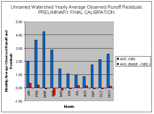
Figure 13 Unnamed Watershed Observed Runoff and Residuals (inches)
Tables 9 and 10 respectively show the simulated and expected water balance for the watershed, and the separate water balances for each land use simulated by the model. As noted earlier, these comparisons are consistency checks to compare the overall simulation with the expected values from the literature, and to evaluate how well the model represents land use differences.
|
Table 9 |
||
|
Expected Ranges |
Simulated |
|
|
Moisture Supply | ||
|
Total Runoff | ||
|
Total ET | ||
|
Deep Recharge | ||
|
Table 10 |
|||||
|
|
Agriculture |
Urban Pervious |
Wetland |
Urban Impervious |
|
|
Moisture Supply | |||||
|
Total Runoff | |||||
|
Surface Runoff | |||||
|
Interflow | |||||
|
Baseflow | |||||
|
Total ET | |||||
|
Interception/Retention ET | |||||
|
Upper Zone ET | |||||
|
Lower Zone ET | |||||
|
Active GW ET | |||||
|
Baseflow ET | |||||
|
Deep Recharge | |||||
CLOSURE
This paper has focused on presenting a 'Weight-of-Evidence' approach to watershed model calibration and validation based on experience with the HSPF model. Examples have been provided to demonstrate some of the graphical and statistical comparisons that should be performed whenever model performance is evaluated. Although not all models will employ the identical procedures described above, it is clear that multiple tests and evaluations, not reliance on a single statistic, should be part of all watershed modeling studies.
REFERENCES
ASTM, 1984. Standard Practice for Evaluating
Environmental Fate Models of Chemicals. Designation E978-84. American Society
of Testing Materials.
AQUA
TERRA Consultants and HydroQual, In., 2001. Modeling Nutrient Loads to Long Island Sound from
Bicknell,
B.R., J.C. Imhoff, J.L. Kittle Jr., A.S. Donigian, Jr, and R.C. Johanson.
1997. Hydological Simulation Program -
FORTRAN, User's Manual for Version 11. EPA/600/R-97/080.
Bicknell,
B.R., J.C. Imhoff, J.L. Kittle Jr., A.S. Donigian, Jr., T.H. Jobes, and R.C.
Johanson. 2001. Hydological Simulation Program - FORTRAN,
User's Manual for Version 12.
Berthouex, P. M. and L. C. Brown. 1994. Statistics for Environmental Engineers. Lewis Publishers, CRC Press,
Donigian, Jr., A.S., 1982. Field Validation and Error Analysis of
Chemical Fate Models. In: Modeling
Fate of Chemicals in the Aquatic Environment. Dickson et al, (eds), Ann Arbor Science
Publishers,
Donigian,
A.S. Jr., J.C. Imhoff, B.R. Bicknell and J.L. Kittle. 1984. Application Guide for Hydrological Simulation Program - Fortran
(HSPF), prepared for U.S. EPA, EPA-600/3-84-065,
Environmental Research Laboratory,
Donigian, A.S. Jr. and P.S.C. Rao. 1990. Selection, Application, and Validation of
Environmental Models. Proceedings
of International Symposium on Water
Quality Modeling of Agricultural
Donigian,
A.S. Jr., B.R. Bicknell, A.S. Patwardhan, L.C. Linker, C.H. Chang, and R.
Reynolds. 1994.
Donigian, A.S. Jr., B. R. Bicknell, and J.C. Imhoff. 1995. Chapter 12. Hydrological Simulation Program - FORTRAN. In: Computer Models of Watershed Hydrology. V.P. Singh (ed). Water Resources Publications, Highland Ranch, CO. pp. 395-442.
Donigian,
A.S. Jr., B. R. Bicknell, R.V. Chinnaswamy, and P.
Donigian,
A.S. Jr., R.V. Chinnaswamy, and P.
Donigian, Jr., A. S., J. C. Imhoff, and J. L. Kittle, Jr. 1999. HSPFParm, An Interactive
Database of HSPF Model Parameters. Version
1.0. EPA-823-R-99-004. Prepared for U. S. EPA, Office of Science and
Technology,
Donigian,
A.S. Jr. 2000. Bibliography of HSPF and Related References. AQUA TERRA
Consultants,
Donigian,
Jr., A.S., 2000. HSPF Training Workshop
Handbook and CD. Lecture #19. Calibration and Verification Issues, Slide
#L19-22. EPA Headquarters,
Donigian,
Jr., A.S., and J.T. Love. 2002. The
Frink, C. R. 1991. Estimating Nutrient Exports to Estuaries. J. Environ. Qual. 20(4): 717 - 724.
HydroQual, Inc. 1996. Water Quality Modeling Analysis of Hypoxia in Long Island Sound Using LIS 3.0. Conducted by direction of the Management Committee of the Long Island Sound Study through a contract with the New England Interstate Water Pollution Control Commission.
Kittle,
J.L. Jr., A. M. Lumb, P.R. Hummel, P.B. Duda, and M.H. Gray. 1998. A Tool for the Generation and Analysis
of Model Simulation Scenarios for Watersheds (GenScn). Water Resources Investigation Report
98-4134.
Lumb,
A.M., R.B. McCammon, and J.L. Kittle, Jr. 1994. Users Manual for an Expert
System (HSPEXP) for Calibration of the Hydrological Simulation Program -
FORTRAN. Water-Resources Investigations
Report 94-4168,
Love, J. T. and A. S. Donigian, Jr. 2002. The
McCuen, R. H. and W. M. Snyder. 1986. Hydrologic Modeling:
Statistical Methods and Applications. Prentice-Hall,
Socolow, R.S., C. R. Leighton, J. L. Zanca, and L. R. Ramsey. 1997. Water Resources Data,
Thomann, R.V. 1980. Measures of Verification. In: Workshop on Verification of Water Quality
Models. Edited by R.V. Thomann and
T. O. Barnwell. EPA-600/9-80-016.
Thomann, R.V. 1982. Verification of Water Quality Models. Jour. Env. Engineering Div. (EED), Proc. ASCE, 108:EE5, October.
Wischmeier, W. H.
and
Zar, J. H. 1999. Biostatistical Analysis. 4th Edition. Prentice Hall,
References
Batty, M. and Xie, Y. (1994a) "Modelling inside GIS: Part 2. Selecting and calibrating urban models using Arc/Info," International Journal of Geographical Information Systems, vol. 8, no. 5, pp. 429-450.
Batty M, and Xie Y, 1994b, "From Cells to Cities" Environment and Planning B 21 S31-S48.
Clarke, K. C. Brass, J. A. and Riggan, P. (1995) "A cellular automaton model of wildfire propagation and extinction" Photogrammetric Engineering and Remote Sensing, vol. 60, no. 11, pp. 1355-1367.
Clarke, K.C., Gaydos, L., Hoppen, S., (1996) "A self-modifying
cellular automaton model of historical urbanization in the
Couclelis H, 1985, "Cellular worlds: a framework for modeling micro-macro dynamics" Environment and Planning A 17 585-596
Debaeke, Ph., Loague, K., Green, R.E., 1991, "Statistical and graphical methods for evaluating solute transport models: overview and application," Journal of Contaminant Hydrology 7 51-73
Gaydos, L., Acevedo, W. and C. Bell. (1995) "Using animated cartography to illustrate global change," Proceedings of the International Cartographic Association Conference, Barcelona, Spain, International Cartographic Association, pp. 1174-1178.
Kirkby, M.J., Naden, P.S., Burt, T.P., Butcher, D.P. (1987) Computer Simulation in Physical Geography. John Wiley & Sons.
Kirtland, D., Gaydos, L. Clarke, K. DeCola, L., Acevedo, W. and
Oreskes, N., Shrader-Frechette, K., Belitz, K., (1994) Verification, Validation, and Confirmation of Numerical Models in the Earth Sciences. Science, vol. 263, pp. 641-646.
United States Geological Survey (1994) Human Induced Land Transformations Home Page: https://geo.arc.nasa.gov/usgs/HILTStart https://geo.arc.nasa.gov/usgs/HILTStart
White, R. and Engelen, G. (1992) Cellular automata and fractal urban
form: a cellular modelling approach to the evolution of urban land use
patterns, Working Paper no. 9264, Research Institute for Knowledge Systems
(RIKS),
Keith C. Clarke, Department of Geology and Geography, Hunter College- City University of New York, and the City University of New York Graduate School and University Center.
Stacy Hoppen, Graduate Student, Department of Geology and Geography,
Leonard J. Gaydos, US Geological Survey, EROS Data Center, NASAAmes Research Center, Moffett Field, CA.
|