Data Integration 3: Digital elevation models

Data Integration 3: Digital elevation models

The earth's surface is a continuos phenomenon. There are various ways of representing such surfaces in digital form using a finite amount of storage. Digital elevation models (DEM) are used as a way of representing surfaces. A DEM is a quantitative model of a topographic surface in digital form. The term digital elevation model or DEM is frequently used to refer to any digital representation of a topographic surface. It is, however, most often used to refer specifically to a raster, regular grid or continuos surface of (spot) heights.

Sometimes the term DTM, Digital Terrain Model, however it mostly refers to a digital representation. Some authors argue that the term ‘Digital Elevation Model’ (DEM) then merely relief is represented, ‘because the term “terrain” often implies attributes of a landscape other than the altitude of the land surface’ (Burrough 1986:39)

DEMs are of great importance to many GIS applications. Inspired by Speight (1974) [SPE.], several researchers describe how topography can be analysed quantitatively through processing of variables that can be derived from digital elevation models.

DEMs provide elevation data for such things as stream flow calculations. Fire risk modelling takes advantage of slope (steepness) and aspect (north-, south-, and west-facing) analysis derived from a DEM. DEMs combined with surface and sub-surface hydrologic data are used for ortho-rectification of digital aerial photography, subdivision planning, road building, overland right-of-way planning, and cell tower placement. DEMs can be used along with radio power data to analyse areas of coverage by radio towers, and to determine the optimum location for new towers. There are obviously many practical applications for DEMs. One very interesting application is to use a DEM to create a shaded relief map base for other digital data. A shaded relief map helps the viewer to really see how roads, rivers, property boundaries, and other map features are situated upon the topography.

From this introduction we expect the student to::

define the term digital elevation model

mention at least two main data structures of digital elevation model

understand the construction of digital elevation models

know six operators to process digital elevation models, In more detail this operators offer the calculation of slope angle, slope curvature, contouring, profiling, mass calculation, vi 111d36b sibility and streaming.

1 Elevation data

'The Earth is not flat, nor is it hollow', defines some of the greatest challenges to describe reality. A geographical information system should provide us with information about vertical surfaces , spiralling phenomena, clusters of points in three-dimensional space and solid masses with caves inside. However this is just a dream.

Nowadays GISsystems are limited to altitude data based on DEMs. Remember that information about altitude given by traditional paper maps looked like figure 1. The picture shows contour data, a set of lines which connect places of equal height.

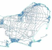Figure 1: Contour data and a derived DEM

Old maps showed already a representation of altitude, but failed to inform about the steepness of slopes, the quantified altitude and the curvature of slopes (Figure 2 )

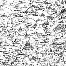
Figure 2: Historical map

In the early 18^th century more detailed maps with height information became available. In countries, like the Netherlands, this information was dedicated to depth of rivers and shallow lakes (fig. 3). From that time on steepness was visualized by using graphic means like a number of small lines (the denser the steeper or the thicker the steeper) that could represent shadow.

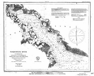
Figure 3 Map with water depths

From geomorphology we know that description of the surface isn't only a matter of points of height but also of structural elements and VIP (very important points). Some of these phenomena (figure 4) are:

spikes, peaks: discontinue heighest point in a certain area, for example a solitary volcano;

pits, sinks: discontinue lowest point in a certain area for example a doline;

watershed delinations : the boundaries of bassins most of the times these are the connected highest points;

drainage pattern : the recognisalbe natural tributaries in an area (watershed);

faults or ridges: an abrupt discontinuity in a certain landscape form for example the San Andreas fault or(US) or the 'Middenpeel' fault in the Netherlands.

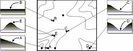
Figure 4: Structural elements and VIP

2 Digital Elevation Model

The abbreviation DEM, Digital elevation model has its origin in the Laboratory of photogrammetry of the Technologic Institute of Massachusetts in the decade of the 50s. In this work Miller and Laflamme (1958) established the first principles of the use of MDT, for the processing of the technologic and scientific problems. The definition of MDT that they speak about in their works is, “statistic representation of the continue surface of the terrain, by means of a big number of points with co-ordinates (X, Y, Z) know, in one arbitrary system of co-ordinates”.

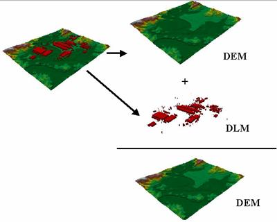
Figure 5: DTM = DEM + DLM

According to literature there are several definitions about Digital Elevation Model (DEM): A digital elevation model is a numerical structure of data that represents the spatial distribution of the land-surface altitude. Besides the term digital elevation model or DEM is frequently used to refer to any digital representation of a topographic surface

Digital terrain model or DTM may actually be a more generic term for any digital representation of a topographic surface.

DEM's of the same area could vary enormously because of differences in the spatial resolution based on the distances between adjacent (grid) points.

3 Data structures

A DEM is a digital description, by data or algorithm, of the surface of an area, Thanks to this the altitude (within a certain accuracy and resolution) of every location can be queried

These are the main data structures that can represent a digital elevation model: (Figure 6; Table 1)

Features Data Structure Specification DEM Storage Structure

Points Lattice Regular points byte, integer, float

Irregular points

Vector Triangular Triangular Irregular topology

Networks(TIN)

Raster Matrix Regular Matrix: equidistant -lattice or Uniform

levels on a square mesh of Regular Grids

rows and columns -Run length

Scalable Matrix: levels in quadtrees

Sub matrices

and of variable resolution

Table 1: Available DEM data structures

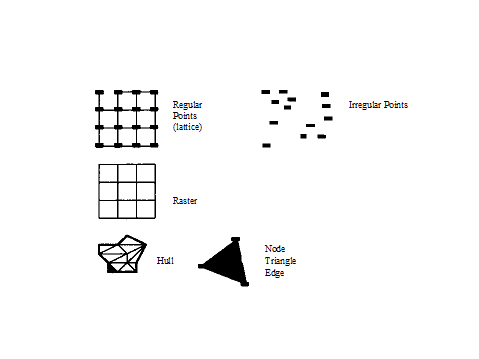
Figure 6: The Data structures for digital elevation model according to Weiber

A variety of data structures for DEMs has been in use over time (Peuker 1978; Mark 1979). Today, however, the overwhelming majority of DEMs conform to one or other of two data structures: rectangular grid (or elevation matrix), or TIN (Triangulated Irregular Network; Peuker,. 1978).

Grids present a matrix structure that records topological relations between data points implicit.

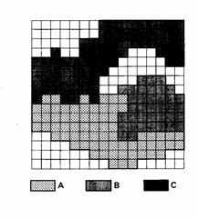
Figure 7 A simple raster DEM

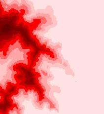
Figure 8 A raster DEM of San Francisco.

Since this data structure shows the storage structure of digital computers, the handling of elevation matrices is simple, and grid-based terrain modelling algorithms thus tend to be relatively straightforward. On the other hand, the point density of regular grids cannot be adapted to the complexity of the relief. Thus, an excessive set of point data is needed to represent the terrain to a required level of accuracy.

Some research, however, reported the use of quadtree method to handle digital elevation data in the grid form so that the data redundancy can be reduced.

TIN structures, on the other hand, are based on triangular elements, with vertices at the sample points.

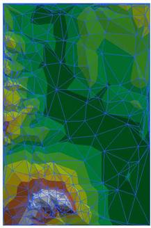
Figure 9 A TIN of Alora (Spain).

TINs are able to reflect adequately the variable density of data points and the roughness of terrain. Fewer points are needed for a DEM of certain accuracy. However, topological relations have to be computed or recorded explicitly.

4 Capturing elevation data

Elevation data can be stored like:

a set of points of height;

a set of contour lines;

a set of triangeld faces (triangulated irregular network);

a regular matrix (elevation matrix).

These data sets can be gathered in different ways:

Digitising and conversion of printed contour lines :

existing plates used for printing maps are scanned

the resulting raster is vectorized and edited

contours are 'tagged' with elevations

additional elevation data are created from the hydrography layer

i.e. shorelines provide additional contours

finally, an algorithm is used to interpolate elevations at every grid point from the contour data

Photogrammetrical:

this can be done manually or automatically:

manually, an operator looks at a pair of stereo photos through a stereo plotter and must move two dots together until they appear to be one lying just at the surface of the ground

automatically, an instrument calculates the parallax displacement of a large number of points

e.g. for USGS 7.5 minute quadrangles, the Gestalt Photo Mapper II correlates 500,000 points

extraction of elevation from photographs is confused by flat areas, especially lakes, and wherever the ground surface is obscured (buildings, trees)

there are two techniques for choosing sample points when using manual

1. profiling

the photo is scanned in rows, alternately left to right and right to left, to create profiles

a regular grid is formed by resampling the points created in this process

because the process tends to underestimate elevations on uphill parts of each profile and overestimate on downhill parts, the resulting DEMs show a characteristic 'herringbone' effect when contoured 2. contour following

contour lines are extracted directly from stereopairs during compilation of standard USGS maps

contour data are processed into profile lines and a regular grid is interpolated using the same algorithms used for manual profiling data

DEMs from each source display characteristic error artifacts

e.g. effects of mis-tagged contours in the products of scanned contour lines

Before properly beginning the operation of the generation of the DEM, the resulting file of the digitalisation must be put under a series of operations of structuring and allocation of attributes that, in summary, are the following ones:

Topologic structuring, by means of which the database is created necessary to maintain and to manage the relation line-node.

Allocation of altitudes to lines and points, since this attribute can not be transferred during the digitalisation.

The generalisation, a selective filtrate process by means of which they eliminate the unnecessary or redundant information in function of the permissible error.

Allocation of codes to the auxiliary structures that have been digitised like complementary information.

Once these operations are made, it is possible to make the creation of the DEMs according to the different methods. The experience has shown that the quality of a DEM can improve significantly introducing auxiliary data of diverse types like, for instance:

Contours that habitually are broken in limited points, mass points, previous generalisation or reduction of the density of vertices of the line.

Singular annotated points or very important points VIPs, these points define excellent information; for example, summits of tips or bottoms of “dolinas”. Sometimes both data types summits and drains must be differentiated clearly due to their different processing.

Structural lines, that define lineal elements with values of altitude associated to each vertex and used to assure the fits of the topographic surface; for example, the fluvial network or lines of crest, this type of lines has frequently been used for the representation of the book land of trips or maps hikers.

Lines of flexion or breakage, breaklines, used to define the position of lineal elements without value of altitude that break the continuity of the surface; for example, cliff edges. These lines do not contribute values of altitude but if they take part in the behaviour of the algorithms of interpolation blocking the search of data. A part of lines of flexion can be extracted from geomorphologic maps.

Zones of constant altitude, defined by polygons that lock up a flat surface of unique height; for example, the surface of a lake.

Zones of cut, which it defines their external limits of the DEM outside of which any existing data is ignored.

Empty zones where the circumstances prevent the obtaining and allocation of levels; for example, flooded zones, snow covers or where the origin data are of doubtful quality.

The data set formed by the mentioned structures can serve to generate a DEM that takes advantage of suitable and effective the topographic information available.

5 DEM construction

The construction of a digital elevation model implies a neighbourhood operation which creates surfaces out of sample points. Another procedure could be started by getting contour data from printed maps ( see 2). However this is a not useful data but the shortage of other source of data obliges to all the GIS systems to have tools to incorporate and use these kind of data. Unfortunately, digitised contours are not suitable for computing slopes or for making shaded relief models and so they must be converted to an altitude matrix.

Unsatisfactory results are often obtained when people attempt to create their own DEMs by digitising contours and then using local interpolation methods like inverse distance weighting and kriging to interpolate the digitised contours to a regular grid. The assumption (spatial autocorrelation) behind the computation of the interpolation weights does not create this problem, but the nature of algorithms. Curiously enough, the more care that is taken to digitise a contour line with many sampled points, the greater the problem explained by Burrough (1986).

The main purpose of constructing a DEM is based on the following proposition.

Given a set of points with co-ordinates (x, y, z), which are distributed irregularly, a regular network will be created by interpolation that represents the real situation with a minimum of information lost.

In the case of the creation of a structure TIN, instead of interpolating, a selection of points is made discarding those that do not contribute an excellent information for the description of the altitude. Nevertheless, in a vector model as the digitised topographic map, to accede directly to a data by its space position is not simple. For this reason, localisation of the data included in the surroundings of the point problem is a key operation that must be well designed given the enormous number of data that usually compose the original map.

According to the interpolation in function of the distance, the value of the point problem is considered assigning weights to the data of the surroundings in inverse function of the distance that separates them from the point problem - to inverse distance weighting, IDW -. Therefore, the nearest points have a greater weight in the calculation, although the relation does not have to be linear.

However making use of the structural elements or very important points (VIP) could improve the quality of DEM that has to be constructed.

The Very Important Points (VIP) at the time of creating a DEM has an importance that is necessary to mention here. In many cases, sample points for a DTM are redundant, i.e. many points can only contribute in a very limited way to describe the surface. Some points, however, are more important since they indicate the 'turning points' of the landform, such as ridges, basins, valleys and slope change points. Using a GIS terminology, these 'turning points' are called VIP. A VIP has the following characteristics:

The slope at a VIP is discontinuous. In other words, a change of slope angle or aspect is expected at a VIP.

If the sample point at a VIP is removed, then there will be significant lost of details about the surface.

The description of a surface can be based on a polynomial function of x_n and y_n that fits all points.

k

H = H (x,y) = a_ij * x_i * y_i

i,j=0

k < (number of points )½

Fitting four points can be done by a 1^st order polynomial:

H = a₀₀ + a₀₁y + a₁₀x + a₁₁xy

And a six points by a 2^nd order polynomial:

H = a₀₀ + a₀₁y + a₁₀x + a₁₁xy + a₀₂y² + a₂₀x²

6 Interpolation

In digital terrain modelling, interpolation serves the purpose of estimating elevations in regions where no data exist. Interpolation is mainly used for the following operations:

Computation of elevations (z) at single point locations;

Computation of elevations (z) of a rectangular grid from original sampling points;

Computation of locations (x,y) of points along contours (in contour interpretation);

Densifying / coarsening of rectangular grids.

Spatial interpolation is the procedure of estimating the value of properties at unsampled sites within the area covered by existing observations in almost all cases the property must be interval or ratio scaled.

Can be thought of as the reverse of the process used to select the few points from a DEM which accurately represent the surface. Also, rationale behind spatial interpolation is the observation that points close together in space are more likely to have similar values than points far apart.

This spatial interpolation is a very important feature of many GIS, in this may be used:

to provide contours for displaying data graphically

to calculate some property of the surface at a given point

to change the unit of comparison when using different data structures in different layers

The quality of interpolation depends on accuracy, number, and distribution of the known points, and how well the mathematical function models the phenomenon.

For example, Lam (1983) [LAM] groups point interpolation into exact and approximate methods. The former preserves the values at the data points, while the latter smooth out the data. Another popular way to classify interpolation models is by the range of influence of the data points involved. Global methods, in which all sample points are used for interpolation may be distinguished from local, piecewise methods, in which, only data points nearby are considered.

1. Point Interpolation/Areal Interpolation

2. Global/Local Interpolators

3. Exact/Approximate Interpolators

Stochastic/Deterministic Interpolators

Gradual/Abrupt Interpolators

Point / Areal interpolation

Point interpolation based given a number of points whose locations and values are known, determine the values of other points at predetermined locations diagram point interpolation is used for data which can be collected at point locations e.g. spot heights.

Interpolated grid points are often used as the data input to computer contouring algorithms once the grid of points has been determined, isolines (e.g. contours) can be threaded between them using a linear interpolation on the straight line between each pair of grid points point to point interpolation is the most frequently performed type of spatial interpolation done in GIS, lines to points e.g. contours to elevation grids

Areal interpolation given a set of data mapped on one set of source zones determine the values of the data for a different set of target zones

Global / Local Interpolators

Global interpolators determine a single function that is mapped across the whole region, a change in one input value affects the entire map.

Local interpolators apply an algorithm repeatedly to a small portion of the total set of points, a change in an input value only affects the result within the window.

Global algorithms tend to produce smoother surfaces with less abrupt changes, are used when there is a hypothesis about the form of the surface.

Exact / Approximate Interpolators

Exact interpolators the data points upon which the interpolation is based on:

The surface passes through all points whose values are known proximal interpolators, B-splines and Kriging methods given data points. Kriging, as discussed below, may incorporate a nugget effect and if this is the case the concept of an exact interpolator ceases to be appropriate.

Approximate interpolators are used when there is some uncertainty about the given surface values.

This utilises the belief that in many data sets there are global trends, which vary slowly, overlain by local fluctuations, which vary rapidly and produce uncertainty (error) in the recorded values.

The effect of smoothing will therefore be to reduce the effects of error on the resulting surface.

Stochastic / Deterministic Interpolators

Stochastic methods incorporate the concept of randomness.

The interpolated surface is conceptualised as one of many that might have been observed, all of which could have produced the known data points.

Stochastic interpolators include trend surface analysis, Fourier analysis and Kriging procedures such as trend surface analysis allow the statistical significance of the surface and uncertainty of the predicted values to be calculated.

Deterministic methods do not use probability theory.

Gradual / Abrupt Interpolators

A typical example of a gradual interpolator is the distance weighted moving average usually produces an interpolated surface with gradual changes.

However, if the number of points used in the moving average were reduced to a small number, or even one, there would be abrupt changes in the surface.

It may be necessary to include barriers in the interpolation process.

As it can see, there are different principles to classify the interpolation methods. Next, the methods of the used software will be described (Arcview-IDW, Spline, Kriging,).

7 Different Interpolation methods are described to continuation:

Spline

The Spline interpolator is a general-purpose interpolation method that fits a minimum-curvature surface through the input points. Conceptually, it is like bending a sheet of rubber to pass through the points, while minimising the total curvature of the surface. It fits a mathematical function to a specified number of nearest input points, while passing through the sample points. This method is best for gently varying surfaces such as elevation. It is not appropriate if there are large changes in the surface within a short horizontal distance, because it can overshoot estimated values.

In ArcGIS, the SPLINE interpolation is a Radial Basis Function (RBF). These functions allow analysts to decide between smooth curves or tight straight edges between measured points. Advantages of splining functions are that they can generate sufficiently accurate surfaces from only a few sampled points and they retain small features. A disadvantage is that they may have different minimum and maximum values than the data set and the functions are sensitive to outliers due to the inclusion of the original data values at the sample points. This is true for all exact interpolators, which are commonly used in GIS, but can present more serious problems for SPLINE since it operates best for gently varying surfaces, i.e. those having a low variance.

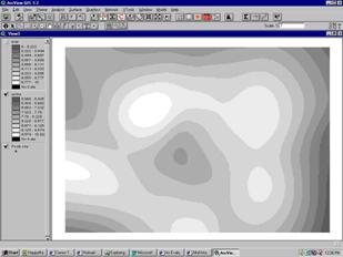
Figure 10   The Spline Interpolation.

Inverse Distance Weighted (IDW)

The Inverse Distance Weighted interpolator assumes that each input point has a local influence that diminishes with distance. It weights the points closer to the processing cell greater than those farther away. A specified number of points, or optionally all points within a specified radius, can be used to determine the output value for each location.

H_R = Σ w_i * H_i / Σ w_i

i

w_i is a certain weight, for example the inverse of the distance between a point and its direct surrounding points

For this method the influence of a known data point is inversely related to the distance from the unknown location that is being estimated. The advantage of IDW is that it is intuitive and efficient. This interpolation works best with evenly distributed points. Similar to the SPLINE functions, IDW is sensitive to outliers. Furthermore, unevenly distributed data clusters results in introduced errors.

An improvement on naively giving equal weight to all samples is to give more weight to the closest samples and less to those that are farthest away. One obvious way to do this is to make the weight for each sample inversely proportional to its distance from the point being estimated.

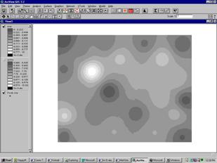
Figure 11:   Result of the Inverse Distance Weighted Interpolation.

Polygonal method

The polygonal method of decluster can be applied easily to point estimation. We simply choose as an estimate the sample value that is closest to the point we are trying to estimate.

The polygonal estimator can be viewed as a weighted linear combination that gives all of the weight to the closest sample value. As long as the points we are estimating fall within the same polygon of influence, the estimate jumps to a different value. The polygonal method shows the discontinuities in polygonal estimates.

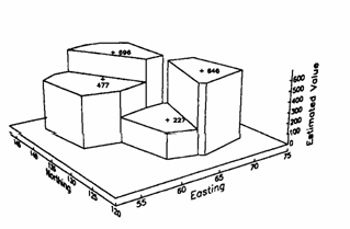
Figure 12:  A perspective view showing the discontinuities inherent in polygonal estimates.

Triangulation

Discontinuities in the estimated values are usually not desirable. This is not to say that real values are never discontinuous; indeed, the true values can change considerably over short distances. The discontinuities that some estimation methods produce are undesirable because they are artefacts of the estimation procedure and have little, if anything, to do with reality. The method of triangulation overcomes this problem of the polygonal method, removing possible discontinuities between adjacent points by fitting a plane through three samples that surround the point being estimated. The expression of a plane can be expressed generally as z = ax + by + c

There are several ways that we could choose to triangulate our sample set. One particular triangulation, called the Delaunay triangulation, is fairly easy to calculate and has the nice property that it produces triangles that are as close to equilateral as possible.

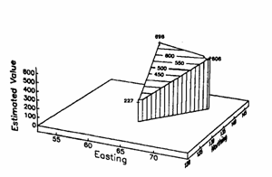
Figure 5.12: Illustration of the estimation plane obtained by triangulation.

Kriging

The kriging interpolator assumes the distance or direction between sample points reflects spatial correlation that can be used to explain variation in the surface. Kriging fits a mathematical function to a specified radius, to determine the output value for each location. The use of kriging involves several steps; exploratory statistical analysis of the data, variogram modelling; then creating the surface and analyzing its optional variance surface. This function is most appropiate when you know there is a spatially correlated distance or directional bias in the data. It is often used to soil science and geology.

Similar to IDW, KRIGING uses weighting, which assigns more influence to the nearest data points in the interpolation of values to unknown locations. KRIGING, however, is not deterministic but extends the proximity weighting approach of IDW to include random components where exact point location is not know by the function. KRIGING depends on spatial and statistical relationships to calculate the surface. The two-step process of KRIGING begins with semivariance estimations and then performs the interpolation. Some advantages of this method are the incorporation of variable interdependence and the available error surface output. A disadvantage is that it requires substantially more computing and modeling time, and KRIGING requires more input from the user. Kriging uses the covariance structure of the field to estimate interpolated values. The resulting interpolated field is optimal in the sense of minimizing the variance among all possible linear, unbiased estimates. Kriging requires a two step process - the fitting of a semivariogram model function (of distance) followed by the solution of a set of matrix equations according to Chao-Yi Lang [CHA.].

Conclusion

Construction of a DEM is based on a number of choices:

the intended spatial resolution;

the number of VIP and structural elements;

the interpolation method (eg. the included number of points)

Many properties of the earth surface vary in an apparently random yet spatially correlated fashion. Using Kriging for interpolating enables us to estimate the confidence in any interpolated value in a better way than the earlier methods do.

Kriging is also the method that is associated with the acronym B.L.U.E. (best linear unbiased estimator.) It is 'linear' since the estimated values are weighted linear combinations of the available data. It is 'unbiased' because the mean of error is 0. It is 'best' since it aims at minimising the variance of the errors. The difference between Kriging and other linear estimation method is its aim of minimising the error variance.

Spline interpolation method is not appropriate if there are large changes in the surface within a short horizontal distance, because of it can overshoot estimated values.

The advantage of IDW is that it is intuitive and efficient. This interpolation works better with even distributed points.

The polygonal method shows the discontinuities in polygonal estimates.

Triangulation method overcomes the problem of discontinuities by fitting a plane through three samples that surround the estimated point. Besides interpolation and including VIP and structural elements are much easier to realize.

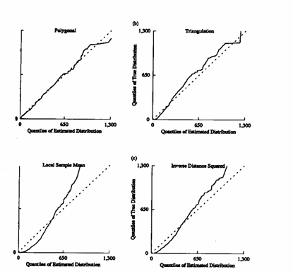
Figure 13   The distribution of the true points values compared to the distribution of the

point estimates provided by the four estimation methods.

Figure 13 helps us to see where the estimated distributions differ from the true one. If the true one. If the true and estimated distributions are identical, then all of their quantiles will be the same and the pairs will plot on the dashed line. If the two distributions have the same shape but different variances, then their quantiles will plot on some other straight line.

Of the four point estimation methods, the polygonal method produces estimated distribution, which is closest to the distribution of true values. Showing that the polygonal estimations have a distribution, which the shape is similar to the true one. All of the other methods produce estimated distributions that are noticeably different from the true distribution.

8 Processing Digital Elevation Models

DEMs provide elevation data for such things as stream flow calculations. Fire risk modelling takes advantage of slope (steepness) and aspect (north-, south-, and west-facing) analysis derived from a DEM. DEMs combined with surface and sub-surface hydrologic data are used for ortho-rectification of digital aerial photography, subdivision planning, road building, overland right-of-way planning, and cell tower placement. DEMs can be used along with radio power data to analyse areas of coverage by radio towers, and to determine the optimum location for new towers. There are obviously many practical applications for DEMs. One very interesting application is to use a DEM to create a shaded relief map base for other digital data. A shaded relief map helps the viewer to really see how roads, rivers, property boundaries, and other map features are situated upon the topography.

According to the succeeding steps to extract information from a DEM three different classes are recognised:

determining attributes of terrain, such as elevation at any point, slope and aspect (first order processing).

finding features of the terrain, such as contour lines, drainage patterns, watersheds, peaks and pits, volumes and landforms (second order processing)

analysing or simulating different elevation dependent interests like hydrologic run off, functions, energy flux, hillshade and viewshed. (third order processing)

8.1 First order processing

Slope calculation

The concept of measuring slope from a topographic map is a familiar one for most professionals in the landscape planning/surveying professions. Slope is a measurement of how steep the ground surface is. The steeper the surface the greater the slope. Slope is measured by calculating the tangent of the surface. The tangent is calculated by dividing the vertical change in elevation by the horizontal distance. If we view the surface in cross section we can visualize a right angle triangle:

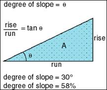
Figure 14

Slope is normally expressed in planning as a percent slope that is the tangent (slope) multiplied by 100. [Percent Slope = Height / Base * 100]

This form of expressing slope is common, though can be confusing since as 100% slope is actually a 45 degree angle due to the fact that the height and base of a 45 degree angle are equal and when divided always equals 1 and when multiplied by 100 equals 100%. In fact slope percent can reach infinity as the slope approaches a vertical surface (the base distance approaches the value 0). In practice this is impossible in a gridded database since the base is never less that the width of a cell.

Another form of expressing slope is in degrees. To calculate degrees one takes the Arc Tangent of the slope [Degrees Slope = ArcTangent (Height / Base)]

(NB. ArcView calculates Slope as degrees)

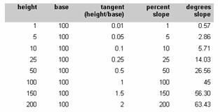
Table 2 Comparison degrees and percentages.

This calculation can be used for every slope of any surface, defined by measures of topography, temperature, cost or other variables. For example you can calculate the slope of the surface defined by air pressure measurements on a weather map to find out where the pressure is changing rapidly—this tells us the location of weather fronts. To continue the same calculation again you can calculate the grade of change by taking the slope of a slope (2^nd derivative of a surface). On a topographic map this is a measure of surface roughness which can be an important factor in estimating the cooling effects of breezes on micro-climates. (Rough surfaces create turbulence and mixing of air masses of different temperatures. This creates better cooling effects at the surface of the ground.

When measuring slope in a GIS the input map must be an interval map that represents a surface as a set of continuous (floating point) values. The output will be on a interval scale.

Methods for calculating slope, aspect and hill shading in a raster GIS

The gradient of slopes is calculated from a 3 x 3 cell window as shown below. The window below represents the eight neighbouring elevations (Z) surrounding the cell at column i row j. Figure 15 shows the window (kernel) used for computing derivatives of elevation matrices. This 3x3 window is successively moved over the map to give the derivatives slope and aspect.

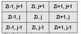
Fig. 15 The window used for computing derivatives of elevation matrices

If average slope is requested, east west gradients are calculated as follows

dEW= [(Zi+1,j+1 + 2Zi+1,j + Zi+1,j-1) - (Zi-1,j+1 + 2Zi-1,j + Zi-1,j-1)]/8dX

The north-south gradient is calculated by

dNS = [(Zi+1,j+1 + 2Zi,j+1 + Zi-1,j+1) - (Zi+1,j-1 + 2Zi,j-1 + Zi-1,j-1)]/8dy

Where

dx = the east-west distance across the cell (cell width)

dy = the north-south distance across the cell (cell height)

Percent slope is calculated by:

Slope% = 100 * [(dEW)^2*(dNS)^2]^1/2

Degrees slope is calculated by

SlopeDegrees = ArcTangent[(dEW)^2 +(dNS)^2]^1/2

Normal GIS Options

Maximum slope is calculated from the maximum gradient of 8 neighbours.

NB. ArcView calculates Slope this way with the result in degrees

Maximum downhill slope is calculated from the maximum gradient of the cell or cells that are less than or equal in elevation to the central cell. If there is no downhill neighbour the cell is assigned a value of -1.

Aspect

Aspect is calculated using the north-south and east-west gradients as expressed in the above equations using the following equation: [Aspect = ArcTangent (dEW/dNS)]

The above equation is adjusted to reflect aspect in degrees in a range from 0 to 360. Where 0 represents a cell with no slope (skyward aspect) and the values from 1 to 360 represent azimuths in clockwise degrees from north. North is 1, East is 90 degrees, South is 180 degrees etc. Optionally, the result is then divided by 45 and converted to an integer to derive a set of generalized solar azimuths range from 0 to 8.

0 - represents non-sloping areas;

1 - represents slopes facing the top edge of a map (North);

2 - represents slopes facing the upper right corner of a map (Northeast);

3 - represents slopes facing the right edge of the map (East);

4 - represents slopes facing the lower right corner of the map(Southeast);

5 - represents slopes facing the bottom edge of a map(South);

6 - represents slopes facing the left corner of a map (Southwest);

7 - represents slopes facing the left edge of a map(West);

8 - represents slopes facing the upper left corner of a map (Northwest)

8.2 Second order processing

Contour line calculation

Contour maps are frequently used to represent surfaces. Contouring produces an output line theme from an input grid or TIN theme. Each line represents all contiguous locations with the same height, magnitude, or concentration of values in the input grid or TIN theme.

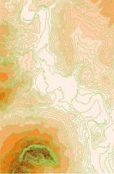
Figure 16:  Example of variable Contour.

Calculation of a contour line is based on the geometrical position of points with a constant value (H = constant). In other words a sectional plane slices the terrain model.

To calculate equal height in a raster you can make use of a linear interpolation. By which H_m gives the average value out of the values of H₁ to H₄.

In a TIN data structure this can be realised by supposing that the end of a line with same height value is located on the edge of each triangle.

(H-H₁) (x₂-x₁)

x_p = x₁ + ----- ----- ----

H₂-H₁

en:

(H-H₁) (y₂-y₁)

y_p = y₁ + ----- ----- ----

H₂-H₁

Profile calculation

Selecting three-dimensional lines from either the graphic or the active theme, users can create profile graphs to see and measure height along those lines. A profile is a vertical section plane of the elevation model. In a raster structure the procedure is as follows (fig. 17):

query the touched and dissected raster cells by the profile line;

calculate the touching or dissecting points and the related heights;

by interpolation in-between points can be calculated.

Figure 17: Profiles in a raster and a TIN (right).

Steepest Path

The steepest path calculates the direction a ball would take if released from a given point on the surface. The ball will take the steepest downhill path until it reaches the perimeter of the surface model or a pit, a point all surrounding areas flow into.

Surface area is measured along the slope of a surface, taking height into consideration. The area calculated will always be greater than simply using the two-dimensional planimetric extent of the model.

Volume calculates the cubic space between a TIN or raster defined surface and a horizontal plane located at any specific elevation.

Volumes are calculated by ::

TIN: Volume = 1/3 Area * (H₁ + H₂ + H₃)

H= height of a triangle vertice

Raster: Volume = 1/4 Area * (H₁ + H₂ + H₃ + H₄)

H = height of 1 raster cel

By changing the base value different volumes for heights or depths can be calculated to realise so-called Cut and Fill analysis. This analysis determines the volumetric difference between two surfaces.

8.3 Third order processing

Hill Shading

Analytical hill shading is a technique for producing shaded relief maps automatically. Relief shading is used to visually enhance the terrain features by simulating the appearance of the effects of sunlight falling across the surface of the land. Hill Shading estimates surface reflectance from the sun at any altitude and any azimuth. The reflectance is calculated in a range from 0 to 100. The equation for the sun in the northwest sky with a 45-degree altitude is as follows:

i)Reflectance = 1/2 + (p’/2) / SQR(po2 + p’2) * 100

where: p’ = (po * dEW + qo * d NS) / SQR(po2 + qo2)

po = 1 / SQR(2)

qo = -po

Hydrological Run-off calculation

Run-off means a peculiar interest in the gravity direction of a certain element (in hydrology the this element is water). Of great importance potential or gravity iso-hypsen which could be derived from slope direction and slope angle.

The algorithm is mostly based on the following procedure:

start with a starting point

calculate gravity points by using the slope angle and the direction of the surrounding areas

if there is no descending area around the procedure stops; either a pit or a sink is the cause of stopping this procedure a new starting point can be initiated!

else the highest gravity point will be selected and the distance between starting point and gravity point will be calculated;

the gravity point become the new starting point.

The calculated runoff direction can be used to find a streaming pattern (eg. Strahler coded) by flow direction or the accumulation of water capacity (fig 18) on certain positions (flow accumulation).

Figure 18: Hydrological calculation results

Visibility studies or viewshed analysis

Viewshed analysis is the study of visibility between points on a terrain surface and used in visual impact assessment. By viewshed analysis, the visibility of every cell (target) from the observer (observer)cell (or numerous observer cells) is computed.

Visibility is calculated by measuring the tangent from the observer's eye to each cell starting from cells closest to the observer. As long as the tangent increases in the line of site from the observer, the cell is visible. If the tangent decreases, the cell is not visible.

The calculation can be tuned by (fig. 19) changing:

local height in a DEM;

view height of the observer;

horizontal and vertical view angle;

view obstacles like buildings, hedges, walls, and so on.

Figure 19: Viewshed analysis variables

Further reading

Weibel, R., Heller, M., 1991. Digital Terrain Modelling. In: Maguire,D.J., Goodchild, M.,

Rhind, D. (eds). Geographical Information Systems. Volume 1: pp. 269-297, Longman

Fisher, P.F.,1996, Extending the applicability of viewsheds in landscape planning. Photogrammetric Engineering and Remote Sensing, 62: 297-302.

Hadrian, D.R., Bishop, I.D. and Mitcheltree, R. (1988) Automated mapping of visual impacts in utility corridors. Landscape and Urban Planning, 16: 261-282.

Klinkenberg, B.,1990, Digital Elevation Models. National Centre for Geographic Information Analysis Unit 38. URL:https://www.geog.ubc.ca/courses/klink/gis.notes/ncgia/u38.html#UNIT38

Sources:

https://www.geog.ubc.ca/courses/klink/gis.notes/ncgia/u38.html

https://www.sli.unimelb.edu.au/gisweb/DEMModule/DEM_Algs.htm

Burrough, P.A., 1986. Principles of Geographical Information Systems for Land Resources Assessment: Chapter 3, Clarendon, Oxford.

Cuberes, S.,2002  DEM's in different geo-information environments, Thesis MSc Geo-Information Science Wageningen

Environmental Systems Research Institute (ESRI) (1996) Working with the ArcView Spatial Analyst.