By William H. Greene
Table of Contents
|
Section Name |
Page |
|
I. What is EA/LimDep | |
|
II. Installing and Starting EA/LimDep | |
|
III. A View of the Desktop | |
|
IV. A Short Demonstration | |
|
V. General EA/LimDep Info | |
VI. The Main Menu | |
|
VII. Using EA/LimDep |
Appendix: Using EA/LimDep
Most of the computations described in Econometric Analysis can be done with any modern general purpose econometrics package, such as LIMDEP, Gauss, TSP, E-Views, etc. We have included on CD as part of the text, a modified version of one of these programs, EA/LimDep, as well as the data sets and program code that were used in the applications in the text.
I. What is EA/LimDep?
EA/LimDep is a computer program that you can use for nearly all the computations described in Econometric Analysis. It is a trimmed version of a large commercial package, LIMDEP (for LIMited DEPendent variable modeling), that is used by researchers in universities, government, and industry for the same kinds of analyses done in this text. There are three differences between EA/LimDep and LIMDEP: First, the size of data sets that you can analyze are restricted to 50,000 values with up to 50 variables and up to 1,000 observations. Second, LIMDEP's very specialized procedures, such as the nested logit model and advanced extensions of the Poisson regression model are not available in EA/LimDep. (You will be able to do all of the computations described in Econometric Analysis save for the more advanced model extensions in Chapters 19 and 20.) Third, the number of parameters in a model is restricted to 15 parameters. (None of the models estimated in the text were larger than this.) In all other respects, this is the full package - it is not otherwise modified or restricted.
This appendix will give a very brief introduction to using EA/LimDep. The full manual for the program has nearly 1,000 pages, so we will only be able to introduce the list of program features. You will have a copy of that manual installed on your computer when 10410h715k you install the program. The Help:Topics feature contains the full manual minus some of the mathematical details. You can refer to this to learn more about using EA/LimDep.
II. Installing and Starting EA/LimDep

EA/LimDep Requires Windows 95, 98, or NT. It will not run in DOS or in
earlier versions of Windows.
To install EA/LimDep, simply place the CD in your D: or E: (CD) drive in your computer. Then, use Start:Run to run D:\Setup to execute the setup program, or click the My Computer icon on your desktop, then make your way to your CD drive, and double click the setup program, or open a DOS window and execute the D:\Setup program. EA/LimDep's setup will take only a minute or two install the program, and does not require you to make any decisions (other than where to put the program, which you can just leave to the setup program). EA/LimDep will occupy about 6 megabytes on your hard disk.
Setup will place a LIMDEP item in your Start:Programs menu. You can invoke the program with Start:Programs:LIMDEP. We find it convenient to put an icon on the desktop to make it easier to start. You can do this as follows: Double click My Computer on your desktop. Make your way to the Program Files folder. You will find an ES folder, and under this, a Program folder. The Program folder will contain an item for LIMDEP.EXE, with a square icon that suggests a plot of the normal CDF associated with the probit model. Single click this icon to highlight it, then drag it to an empty place on your desktop.
The first time you invoke EA/LimDep, you will be asked to 'Personalize' your copy. This is not a registration; you are just putting your name on your program. There are no serial numbers, no keywords, and no registrations for EA/LimDep. This is free software. In fact, after you install it on your computer, we hope you will pass your CD on to someone else, so that they can install it on theirs! (There are a number of data and program files on the disk, so be sure to copy these to your own hard disk before you pass on the CD.)
![]()
Because EA/LimDep is freeware, we are not able to provide technical support for it.
III. A View of the Desktop
When you start EA/LimDep, your desktop will appear as follows: (The 'command window' below the row of buttons may not be present. To install it, click Tools:Options:View then click in the check box next to 'Display Command Bar' and finally, click OK. This setting is permanent until you change it.)
HINT: Do not ever
'close' this window. You must have a
project window open for the other functions of the program to operate.
Click here for
the
File:New menu
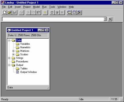
EA/LimDep uses a standard Windows style statistical package, three window mode of operation. The first window you will see is called the 'project' window. A project consists of the data you are analyzing and the results of your computations, such as estimates of coefficients, other matrices you might have computed, and so on. As we'll see shortly, this window contains an inventory of the things you have computed - that inventory will grow as you manipulate your data.
The second main window that you will use is the 'editing window.' This will be the place where you put your instructions to EA/LimDep As with any Windows program, EA/LimDep makes use of many menus and dialog boxes. However, you will find at some point quite soon that the menus are too slow for what you wish to do, and you will switch to a command format in which you type out your instructions to get the program to do computations such as regressions. We'll demonstrate shortly.
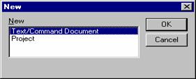
Open an editing window by clicking File:New to open a 2 item dialog box. The item highlighted is Text/Command document, which is what you want, so just click OK to open the editing window. This will usually be your first step after you start EA/LimDep.
Your desktop will appear as below after you open your editing window.
You will type your
commands in this
window
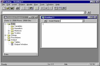
This window is the 'input' window. You are now ready to start using EA/LimDep to analyze data or do other computations. You will put your instructions in this window. When you (the program) carry out the instructions, the numerical results will appear in the third main window, the 'output' window. The output window is created automatically for you when you issue a command. We'll look at an example below.
There will be many other 'transient' windows that you will open and close. For example, when you produce a plot or use matrix algebra to produce a result, or when you enter data by reading a spreadsheet, you will use one or another sort of window which you will open, then probably close as you move on to your next computation or operation. The three primary windows, project, input, and output, will usually stay open on the desktop at all times. No doubt you will size them and move them around to arrange the desktop in a way you prefer.
IV. A Short Demonstration
We're ready to get started. Before working through an organized 'minimanual,' let's illustrate operation of the program by carrying out a small application from beginning to end. Table A6.1 lists a small data used in several of the examples in Chapter 6 The data are listed below.

Year GNP INVS CPI i
873.4 133.3 82.54 5.16
944.0 149.3 86.79 5.87
992.7 144.2 91.45 5.95
1971 1077.6 166.4 96.01 4.88
1972 1185.9 195.0 100.00 4.50
1973 1326.4 229.8 105.75 6.44
1974 1434.2 228.7 115.08 7.83
1975 1549.2 206.1 125.79 6.25
1976 1718.0 257.9 132.34 5.50
1977 1918.3 324.1 140.05 5.46
1978 2163.9 386.6 150.42 7.46
1979 2417.8 423.0 163.42 10.28
1980 2633.1 402.3 178.64 11.77
1981 2937.7 471.5 195.51 13.42
1982 3057.5 421.9 207.23 11.02
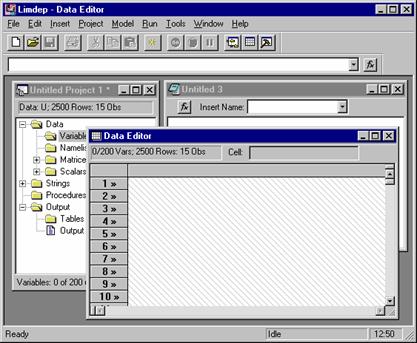
Our first step is put these data in the program in a place where we can use them. There are many ways to do this, including importing from another program, such as Microsoft Excel. We'll begin from scratch, and type them in directly. (This will take a few minutes, but it will familiarize you with an important part of EA/LimDep.) The button second from the right at the top of your screen (with a grid icon) activates the data editor. When you first activate it, the data editor is empty. You wish to put five new variables in it. Step 1, then, is to press the right mouse button to activate a menu which will create a column for you to put data on a variable into.

Select this item to create a new variable in the project. Press the right mouse button to activate this menu New Variable... Import Variables... Export Variables... Sort Variable... Set Sample > Split Window![]()
![]()
![]()
![]()
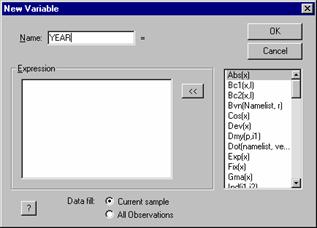
When you select 'New Variable,' a dialog box will appear. This box allows you to create a column in your spreadsheet for a variable. We've typed the name YEAR in the name field. Then, press OK - there is no need to enter a formula - though you can if you wish.
Press OK after you enter the name of the new
variable. This is a list of the
mathematical functions that are available for transformations of variables. You can define a formula for
a transformed variable in this
window. Hint: If you press this button, you will activate the Help feature. This opens the electronic
manual.
![]()
We repeat this for each of our 5 variables. The data editor will be reformatted as a grid, and we enter the data on our five variables. The end result appears as follows:
Use the usual editing keys, ,
, . ,
Enter, Backspace, and so on to move around this
spreadsheet style data editor. Enter
values as you would in any spreadsheet program. When you are done entering data, just
close the window by clicking . Or, just minimize it, in case you want to
come back later. Hint:
This window is updated automatically. All variables that exist are in this window at all times, regardless
of how or when they are created.
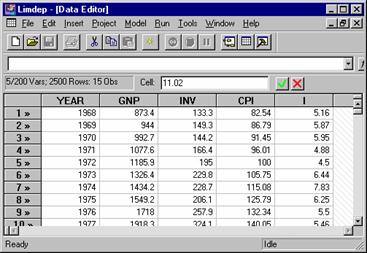
Before moving on to the analysis, we close the data editor by double clicking the grid icon at the upper left of clicking the ' ' box at the upper right of the editor (not the topmost one, which closes the whole program). We now have five variables in our project. Notice that the project window has changed to reflect this: The original project window that came up when we started showed nothing next to the 'Variables' item. Now, by clicking the '+' box next to 'Variables,' we find the list of our 5 variables.
Click this + box to display the list of variables that exist.![]()
![]()

The raw data are ready to analyze. In order to carry out the computations in the examples in Chapter 6, it is necessary to transform the data to
y = Real Investment = (Inv/CPI)/10 (trillions),
X = x1 = Constant term equals 1 for each observation,
x2 = Trend,
x3 = Real GNP = (GNP/CPI)/10 (trillions),
x4 = Real Interest Rate = Interest - Inflation,
x5 = Inflation Rate = 100%[(CPIt - CPIt-1)/CPIt-1] with CPI0 = 79.06 from a footnote.
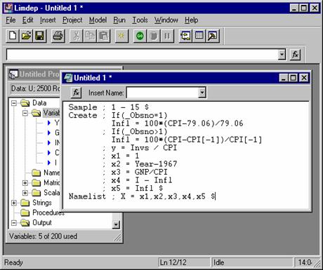
As in all cases, there are many ways to do these computations. The method you will use most is to put the necessary instructions in your input window, and have them carried out by the program. The steps are shown below. The instructions needed to do these computations were typed in the editing screen. (The screen is 'activated' first by placing the mouse cursor in it and clicking once.) Notice that there are three instructions in our editor. The instructions are:
SAMPLE explicitly defines the current sample to have 15 observations;
CREATE defines the transformed variables that we want in our X matrix;
NAMELIST defines a matrix named X which contains these 5 variables.
Each command begins on a new line, and consists of a verb followed by a semicolon, the instructions, and a dollar sign to indicate the end of the command. The steps needed to 'carry out' the commands once they are typed are shown with the figure. Capitalization and spacing do not matter. Type the text in any fashion you like, on as many lines as you wish. But, remember, each command starts on a new line.
Step 1: Click Edit: Select All. This will 'select' the commands in the screen. You can also select only some by using your mouse. Step 2: Click the GO button. This will
'submit' your commands. They are then carried out.
This is the command bar
![]()
![]()
![]()
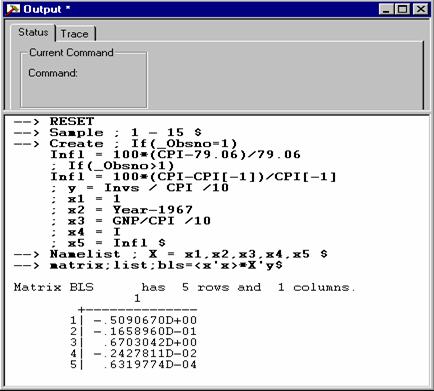
In Example 6.8, we computed a vector of regression coefficients by the familiar least squares formula b = (X X)-1X y. Before we do this, there are a few points we must note. First, every computer package which does this sort of computation has its own way of translating the mathematical symbols into a computerese that it understands. You cannot type the necessary superscript to tell EA/LimDep to invert X X (or any other matrix). The symbol for this is <X'X>. Second, there is an important footnote under Table 6.2. It says that you will get different answers if you use the internal values at full computer precision rather than using the rounded values that you see in the table. We're about to see that the difference can be large. This is a consequence of rounding, not an error. Continuing, then, here is another way to compute a result.
Step 1: Put the mouse cursor in the command bar and click. (See the figure above).
Step 2. Type MATRIX ; List ; BLS = <X'X> * X'y $ then press the Enter key.
Your output window will contain the results. Some things to note: EA/LimDep often uses scientific notation when it reports results. The value -.1658960D-01 means -.1658960 times 10-1, or -0.01658960. Let's compare these to the results in the text. The first four values are close, but not identical. But, the last is fairly far from the value in the text. Once again, this is a result of the rounding that produced the table in the text. This explains the footnote in the text. To verify this, you might repeat this exercise beginning with the transformed data given in table 6.2.
Finally, we consider a menu driven way to enter instructions. Matrix algebra, transformations of variables, and calculator computations involve infinite numbers of different things you might do, so they do not lend themselves to using menus. A menu structured variable transformation program would be intolerably slow, and would necessarily restrict you to a small part of the algebra operations available. But, specifying a regression model is much simpler. This need involve nothing more than pointing at the dependent variable and a list of independent variables. EA/LimDep allows just this sort of approach in specifying a model.
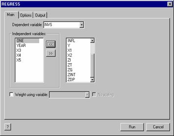
The dialog begins with Model:Linear Models:Regression... A dialog window will appear next: The model dialog window typically has two or three tabs, depending on the model you will be specifying. For the linear regression model, there is a Main page, on which you select the dependent variable and the independent variables. After you do this, you can either submit the simple specification, by clicking Run, or you can add other optional specifications. For the one shown below, the main page specifies the dependent and independent variables for a linear model, while the Options page will allow you to specify an extended model with autocorrelation, or to specify computation of a robust covariance matrix.

You can access the manual, with a full description of the model and how to estimate it, by clicking the '?' icon at the lower left of this dialog box. This will be true in many other dialog boxes that EA/LimDep presents.
Press Run to
estimate the model. To select the independent
variables, including the constant, select each variable from the vertical
list, then press the <<
button to move that variable into your list. You can do this in the other direction if
you need to correct an error. Hint:
Double clicking a name will move it to the other window. To specify the dependent variable, click the menu button
then select the variable.![]()
![]()
![]()
![]()
![]()
This presents a new set of results in your output window.
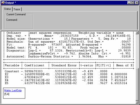
This concludes the demonstration. You can now exit the program with File:Exit.
V. General EA/LimDep Info
This and the next several sections will show you how to operate EA/LimDep and how to use it to do the computations described in the text. This will only be a brief introduction. The Help:Topics file provided by the program provides roughly 800 pages of the full manual for the program, including many chapters on specific topics in econometrics. So, once you get started here, you should refer to that document for more information about operation and topics such as heteroscedasticity and autocorrelation.
We will consider three levels of discussion in this discussion:
1. How to operate EA/LimDep. This includes how to use the menus, using files, and so on.
2. The program command language. This part will describe how to instruct EA/LimDep to carry out
operations, such as compute a transformed variable, do matrix algebra, or estimate a model.
3. Specific commands and instruction. This section will describe specific applications described in the
text, such as computing a restricted regression, estimating a heteroscedastic regression by weighted
least squares, and so on.
Before proceeding with any of these, it is necessary to describe in general terms the overall design of the program. (We'll be brief.)
When you use EA/LimDep, you will analyze a 'project.' A project consists of all the things that you create as your session proceeds. As you saw at the beginning of Section III, your computing session begins with an empty project, indicated by the project window with title 'Untitled Project 1.' You will usually begin your session by doing one of two things: (1) 'Loading' a previously created project, so that you can continue an earlier session. (This will probably become your most frequent starting point), or (2) beginning a new project by reading or moving a data set into EA/LimDep's workspace so that it can be analyzed. The data that you analyze are part of the project. As your session proceeds, you will accumulate matrix results, for example, every time you estimate a model, and you will define other things such as groups of commands called procedures, scalar results that you compute, such as an F statistic, and so on. All these entities that you create become part of the project. You may only analyze one project at a time.
There is only one project window. This window contains an inventory of the things in your project, such as variables, matrices, procedures, and so on. As you proceed, you will also open and close other windows. As described earlier, there are three main windows on your desktop, the project window, the editing, or input window, and the output window. Commands go in the first of these; numerical results that are created by your commands will be placed in the second. Descriptions of these, including pictures, are shown in Section IV of this guide. You may also create a variety of lesser windows as you proceed. The data editor that we examined earlier is one. Each time you produce a plot, for example a histogram, the figure will be placed in a window. If you wish, you can open a separate window for doing matrix algebra computations. And so on. Most of these windows are 'transient.' You will use them for a purpose, then close them fairly quickly. Normally, however, you will keep the three main windows open. It is necessary to define the active window. This is simply the window upon whose contents you are operating on at any point in tiem. Notice, for example, in the first figure of Section IV, there are three windows open. The data editor happens to be at the forefront, but only because we sized it to be that way. However, the data editor is also the active window in this figure. You know this because the title bar of the Data Editor window is dark whereas the title bars in the other windows are light. This is important, not only for the obvious reason that you cannot operate on a window or use the features in it unless it is the active one, but also because certain menu functions are only available in certain types of windows. Thus, for example, the Edit menu contains many functions that are unavailable when the output window is the active one. You can activate any window just by clicking your mouse anywhere in that window.
VI. The Main Menu
This section will describe basic
operation of the program. This will
center primarily on the menus and buttons at the top of the desktop. Section VII will discuss specific operations,
such as how to read a file.
The Main Menu, Buttons, and Command Bar
|
|
|
|
Open new editing or project window
Close the active window (editing or output)
Standard Save and Save As... functions to save
the current project, editing, or output window in
a file. Also saves plots as .WMF (metafile) files.
Reload previous project or save the current one
in a file (will be called NAME.LPJ).
Use for printing contents of editing window,
output window, or a high resolution graph
Previous four editing files. When you select
one of these, it is placed in a new editing window
Previous four project files. When you select one of
these, the session is restarted with this new project
End the session and close the program.
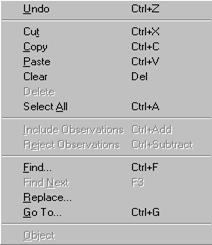
Standard editing functions
used in the editing, input window. You can also cut, paste, and copy among editing, output, and various
calculator (matrix, scalar) windows. You can also copy and paste from any window to other software, e.g.,
from the data editor into Excel or output to Word. Include and Reject menu items
are only used when the data editor is active. Use to mark observations in or out of
current sample Navigate editing window
Edit
Insert
|
|
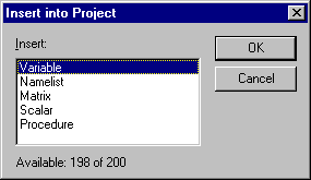
Insert things into the
editing window. Text file places a
whole text file in the window. Insert Item into Project is a powerful processor that starts several
operations.
Program parameter settings such as data area size and
where to put the trace file.. You should not use this.
Project
Clear all work areas. Retarts the project. Deletes
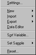
all data! Use with care. Sort observations in a column of data into ascending or
descending order. You can also carry other variables with the one you sort. Same as Insert Item into Project. Use Import to read a data file. Use
Export to write a data file for some other program. Data Editor activates the data editor for
entering new variables or editing existing ones.
Model
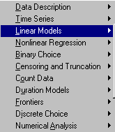
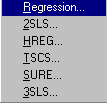
Use the model menu to specify a model in a dialog box instead of a command. The main page specifies the essential parts, usually the dependent and independent variables. Other pages are for options and extensions, such as heteroscedasticity robust covariance matrices, autocorrelation, or fixed effects.
|
|
|
|
Run
Used with the text editing
window. Run line and Run Line
Multiple times submit a particular line that you have highlighted to the
program for execution, once or more than once. Run file executes a set of commands that
are stored in a command file. This
is the same as Insert:File, then Select All and GO. New Procedure is an interactive editor
for procedures. This is an advanced
feature. See Chapter 37 of the
manual for details.
Invokes windows specific for
the scientific calculator and for matrix algebra. These are just convenient windows for
arranging results of these operations. Review tables is used for setting up results of model commands. Tools:Options is used for program
settings, some the same as in Projedt Settings. This should generally not be needed.

Window
|
|
These are the standard
Windows functions for arranging the desktop or activating a particular
window. The list at the bottom is a
complete inventory of the windows currently open. The first two are the project and editing
window, respectively. Asterisks
indicate that the open window has changed since it was last saved. When you exit the program, you will be
asked if you would like to save any window which is open and has been
changed since the last save (or since it was opened).
Help
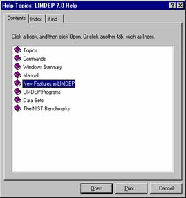
Help contains the full manual
for LIMDEP as well as several other summaries and descriptions. The Commands
book contains details on each program instruction. The Topics book includes descriptions of
specific operations such as how to read a data set.

VII. Using EA/LimDep
This section will provide the information you need to use EA/LimDep to analyze your data and to do the other computations described in Econometric Analysis. The descriptions will be extremely brief; only the essential features will be described. There are many features of the program that are available to you that will not be mentioned here. However, your Help file contains the full manual for the program, so you can find the additional descriptions there. Do note that since the online manual is the documentation for the full commercial version of LIMDEP, many of the model estimation features described in there are not available in this restricted version.
A. Starting, Ending, and Restarting Your Session
As we showed in the tutorial, you start EA/LimDep either from the Start:Programs menu or from the LimDep shortcut icon that you placed on your desktop. To end your session and close the program, use File:Exit. When you exit, you will be asked if you would like to save the contents of the active windows that have changed during your session. Usually, the first such query will be this one:
This is the program's 'system save' feature. By saving the changes to your project,
you can restart your session later by selecting this project from the File menu. 'Unititled Project 1' is the default name
for the project file. You may use
some other name if you prefer. As a
general rule, you should save your project when you exit the program. Project files receive names that end with
a .lpj suffix.

You will also be asked if you wish to save 'Untitled 1' (or some other name if you have changed the default.) This will be the text editor window. The text editor window is not saved in the project. (The reason is that you may have multiple editing windows open if you wish.) If you wish to save the contents of the editing window for later, you should use this feature now. Editing files are saved as .lim files.

Tip: The .lpj and .lim file types are entered in your Windows registry. If you save one of these file types to your desktop, you can use it as a shortcut to launch EA/LimDep. By double clicking a .lim or .lpj file in any context, you can launch EA/LimDep and then automatically open an editing or project window.
When you wish to restart a
session, if it is one of the most recent four projects that you saved, you
will find the project listed at the bottom of the File menu. You can
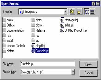
just select the name from the menu (one click) to reload the session. If it is an older session, use File:Open Project to locate and open the
.lpj (or .sav) file. Text editing
windows are restored the same way. The File menu contains the
last four saved .lim files above the .lpj files in the menu. If the one you
want is not in the list, use File:Open
to locate it. This will
automatically open the file and put its contents on your screen in an
editing window.
B. Commands, Syntax, Names
Many of the operations you carry out will be done with menus. However, almost all the instructions that you give that involve analyzing your data, matrices, the scientific calculator, or any kind of programming that you may do, will be submitted to EA/LimDep by typing them on the screen in your editing window or in a command window in some context. There are a few conventions that you will need to know about as you create sets of instructions in your editor:
(1) Commands are of the form VERB ; specification ; specification ; ... ; ... $
The verb is a command such as READ or REGRESS. Specifications are specific to the context. The
internal delimiter is the semicolon character. All commands end with a dollar sign.
![]()
Tip: If you submit a command and 'nothing happens,' check to see if you forgot the ending $.
(2) The order of the specifications in a command never matters.
(3) Case and spacing never matter in any instruction. You can type commands in any way that you
prefer. Use spacing and upper and lower case to make your commands easy to read.
(4) Every new command which begins with a verb must begin on a new line.
(5) Any line that begins with a question mark, regardless of where it appears, is treated as a comment and
not used in any function. This allows you to put comments in your command sets.
The fifth window shown in the demonstration in Section IV above shows an editing screen which contains a sequence of three instructions, Sample, Create, and Namelist, that follow these conventions. You can obtain a full list of the verbs used in EA/LimDep in the online Help file in the 'Commands' book.
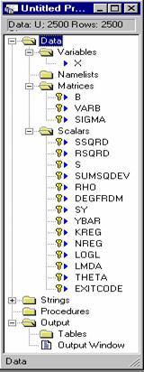
Many of the computations that you do will create numeric entities that have names. For example, your data set will consist of n rows, or observations, on a set of variables, which will have names so that you can refer to them later. There are a few 'reserved' names in EA/LimDep. These are reserved for use by the program for results that are saved automatically when you estimate a model. You can see the list of these in your project window:
Reserved names are always
marked with keys (to indicate that they are 'locked.') The variable X is our own. Notice
that it is unmarked. The name ONE is used to indicate the
constant term in a model. This is
not a valid variable name, either, though it does not appear in the project
window. You will be warned if you
try to use a reserved name. These three matrices are
created by the program and are reserved. You can use matrix algebra to create other matrices with names that
you choose. These are scalar values that
are created when a regression or other model is estimated. These names are also unavailable for
other uses. You can use the
calculator to calculate other values that you can give a name to, so that
you can use it in some other expressions. Two other names that are used by the program are N, the current sample and PI, the number 3.14... The project window will
always contain a full inventory of the named entities that exist in your
project. This window is more than
just a listing, however. By double
clicking any name in the project window, you can invoke some processor that
is relevant to the name you selected. For example, if you double click a variable name, you will invoke
the data editor. If you select a
variable name, then click the right mouse button, a different menu of functions
is offered. There are many other
functions embedded in the project window that you can start by clicking the
different names in the lists. Section 3.5.2 of the manual contains details.
Names that you create must all obey the following conventions:
(1) They must contain from 1 to 8 characters. No name may contain more than 8 characters.
(2) Names must begin with a letter. Numbers and underscores may appear after the initial letter.
(3) Names may only use the 26 letters, 10 digits (0 - 9), and the underscore character. Any other character
in a name is likely to cause problems elsewhere, though in most cases a bad name will be noticed.
(4) Since case never matters, you cannot create different names by using different cases. Bob = BOB.
C. Submitting Commands
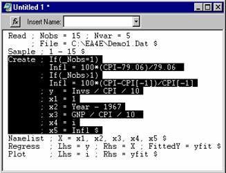
In order to submit commands, type them onto the text editing screen, drag your mouse across the ones you wish to submit to highlight them, then press the GO button at the top of the screen. Or, to submit the entire screen contents at once, use Edit:Select All, then GO.
At the left, we have a screen
with a number of commands, but at this point, we are only going to execute
the Create command. Later we can go back to submit the
others. The advantage of this method
is that the commands remain in the editor if you wish to use them again. For example, the Regress command has an error in it. 'FittedY='
is supposed to be 'Keep='. When we submit it, this command is going
to result in an error message, but no results. So, we just go back to the editor, fix
the error, and try again.
D. Reading a Data File
Step one in analyzing a data set will be to read it into EA/LimDep's data area. One way to enter data will be to type them in the data editor, as we discussed in the demonstration in part IV. You can read many kinds of data files. We will consider two, spreadsheets and rectangular ASCII files. You can read about others in Chapter 5 of the online manual.
(1) To read a spreadsheet file that you have written with Microsoft Excel (.XLS style file) or Lotus (.WK1 style file), or any other program that will create a spreadsheet file of one of these two types:
a. Make sure that the first row of your spreadsheet contains valid variable names as column headers. Then save the file using the usual procedures.

IMPORTANT NOTE: If you are saving a spreadsheet file with Excel, use Save As... and save the file as type Microsoft 4.0 Worksheet *.xls. EA/LimDep cannot read the default format file created by Excel but it can read a type 4.0 worksheet.
b. Use Project:Import/Variables from the main menu, or open the data editor, then press the right mouse button, and select Import variables. In either case, use the file navigator to find, then select the file and just Open it. The data will be read into the program, and will be ready for you to analyze them.
(2) To read a rectangular ASCII file:
a. First create the file with any text editor. The contents must be ASCII (text) data. You should put a row of variable names at the top of the file. The sample data set shown at the beginning of Section IV is precisely in this form. Be sure that the names at the top of the file and the values in the file are separated by blanks and/or commas. You can use more than one line for the names if necessary.
b. In order to instruct EA/LimDep to read this type of file, you must use a typed instruction in the text editor. If an editor window is not open already, use File:New/OK, then activate it. Place the command
Read ; File = ...<name of the file>...
; Nvar = the number of variables ; Nobs = the number of observations
; Names = 1 (or the number of lines of names that appear at the top of the file) $
on the screen. Now, highlight these lines with your mouse either by dragging the cursor over them or using Edit:Select All. Then, press the GO button at the top of your screen.

IMPORTANT NOTE: If your file contains missing values, you must put something in that place in
the file to indicate so. Blanks are just space between numbers. The word 'missing' will suffice for this
purpose, as will a simple '.' with spaces on either side of it.
If you need to locate an ASCII file to put its full name in your READ command, you can use Insert:File Path from the main menu to navigate to it. This will type the name in the editor screen for you.

NOTE: If your ASCII data file contains exactly one row of names at the top of the file, followed
by a simple data set with values separated by spaces and/or commas, then you can read the file with
the simple command READ ; File = ...<name of the file> ... $ or just by pointing at it with
Project:Import/Variables. This will be the usual case, so this is how you should open a data file.
If you would rather not use several pieces of software, or are unfamiliar with other programs that can be used to edit an ASCII data file, here is a convenient trick that we often use to get ASCII data into the program and create the data file at the same time. You can READ data directly off the editor screen.
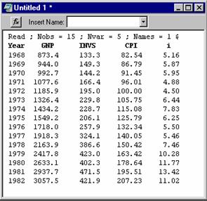
The data used in the demonstration could be read as follows:
Step 1 is to type the command shown, the names, and the data on the screen in the text editor. We have neatly arranged the columns, but this is not necessary, so long as values are separated by blanks and/or commas. Step 2, is to READ the data, which we do with Edit:Select All, then GO.
This can also be written as a text file just by saving the window. Use File:Save. If you do not have any other convenient text editing program, the text editor in EA/LimDep can be used for that purpose. The editing conventions and keystrokes are all the standard ones used in Windows applications.
E. Transforming the Data
Once your data are placed in the program work area for use, there are two steps remaining that you will usually take before actually doing estimation. First, you will usually want to create transformed variables, and, second, you will often want to use subsets of your observations.
To obtain transformed variables, such as squares, logs, products, and so on, use the text editor to submit the instruction, or open the data editor, press the right mouse button, and select New Variable. The expression you will use is the same in either place. The command for computing transformed variables is
Create ; name = expression ; name = expression ; ... ; name = expression $
for as many transformations as you wish. The command may transform an existing variable, such as X=100*X or it may create a new one, such as LogX = Log(X). The expressions can be any algebraic expression involving +, -, *, /,. or ^ (for raise to the power), as many levels of parentheses as you need to get the right result, and any variables that exist in your data set. Functions include log, exp, abs, and nearly 100 others. Chapter 5 in your online manual contains a complete list of the available functions for transformations of your data and details on some other useful operations.
A transformation can be made conditional by putting the condition in parentheses. For example:
Create ; If (Age < 21) Minor = 1 ; (Else) Minor = 0 $
(Note: Create;Minor=(Age<21)$ is equivalent.) There are dozens of specific transformations that you can use. Some that you are likely to find useful are:
Standard functions: Log(name), Exp(name), Abs(name), where name is the transformed variable.
Random numbers: X = Rnn(mu,sigma) (where you give the two values), computes a column of
random draws from the normal distribution. You can operate on these values
as well. Thus, chisq = (Rnn(0,1))^2 is the square of a standard normal.
Trends: Trn(a,b) = a, a+b, a+2b,... so, Trn(1,1) = 1,2,3,...
Strata: Trn(m,0)=1,1,...(m times), 2,2,..., 3,3,... and so on. Trn(4,0)=1,1,1,1,2,2,2,2,..
Dummy variables: Minor = (Age < 21) is the same as the command above.
WrkWoman = (Female=1) * (Income > 0) creates a dummy variable = 1 if
both conditions are true. Operators are <, >, <=, >=, =, and # for not equal.
There are many other functions and variations available for transforming data. Further details appear in Chapter 5 of the manual.
F. Setting the Current Sample
The 'current sample' is the set of observations that is used in any operation that involves computing something using your data. Normally, this will be all the observations in your data set, but it might not be. You might wish to set the sample as something else. The commands are:
Specific Observations: Sample ; i1 - i2 $ Uses observations i1 through i2. If you read a data set with 15 observations, the current sample is set automatically to 1 - 15. Suppose you want to compute a regression with observations 3 to 12. you would use Sample ; 3 - 12 $ After you issue this command, all subsequent computations involve observations 3 to 12. Restore the full sample with Sample ; All $
Deleting observations: Beginning with a particular sample, you can delete observations from the sample with Reject. For example, to analyze the women in a sample, you could use Reject ; Male = 1 $ After you operate on a subset of a sample, you will probably wish to continue operating on the full sample. Restore the full sample with Sample;All $
If you have time series data, you can use the dates in sample setting commands. This requires two parts. You must first indicate that your data are time series with a Date command that identifies the first date in your data. The syntax is Date;year$ if the data are yearly (e.g., Date;1951$); Date;Year.q$ if the data are quarterly, where q is, 1, 2, 3, or 4 (e.g., Date;1953.1$); or Date;Year.mo$ where mo. is 01, 02, ..., 12, if the data are monthly (e.g., Date;1960.01$). Once this is done, the Period command is used to set the current sample. The Period command appears as Period; first date - last date $ For example, Period;1960.01-1995.12$ (No, EA/LimDep does not have any 'Y2K' problems.)
G. Lists of Variables.
Many of the computations you will do with EA/LimDep will involve sets of variables, and frequently, you will use the same set of variables more than once. There is a simple tool you can use to make this easier, the Namelist command. The command is
Namelist ; name = list of variable names $
Thereafter, the name on the left hand side stands for the list of names on the right. An example appears in Part C above; Namelist ; X = x1,x2,x3,x4,x5$ is followed by a Regress;...;Rhs=X$. This specifies a regression of a dependent variable on the five variables in X. You will see many applications that use this tool. You can have up to ten namelists defined at any time. They may share names. Thus, for example, Namelist;XYZ=X,y,z$ is a valid definition of a namelist that stands for seven names, the five in X plus y and z.
H. Summary
You now have all of the basic tools needed to operate EA/LimDep. There are four features remaining to describe, estimating models, using matrix algebra, using the scientific calculator, and writing procedures. Before turning to these, we provide a small application which uses the features described above.
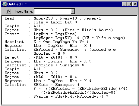
We will use a data file called Labor.Dat to fit a log-linear hours equation. These data are a set of 250 observations on women's labor supply, which are provided in Berndt (1992). Just for illustration, we will carry out a Chow test of the hypothesis that the labor supply behavior of women with children in this sample is the same as that of women without children. The sample is divided into two groups of women, one group that did not participate in the labor market and one that did. To carry out our test, we will restrict our attention to those in the latter group. The regression equation we will use is
log(hours) = b1 + b2log(wage) + b3Age + b4Educ + e.
The editor screen is shown below. We would execute all the commands on the screen at once, and collect the results we need at the end.
![]()
Once your data are in place, you are ready to use the program tools to do the analysis. For direct manipulation of your data and related computations, you will use four sets of program features.
A. For data description and model estimation, you will use large preprogrammed 'routines' such as the REGRESS command. These single commands produce large amounts of numerical output including estimated parameters, standard errors, and associated statistics such as fit measures and diagnostic statistics. Chapters 12 through 33 of the online manual describe the roughly 50 estimation procedures contained in the full package. The following subset those routines are provided in EA/LimDep:
Descriptive Statistics
DSTAT descriptive statistics,
HISTOGRAM histograms for discrete or continuous variables,
PLOT/MPLOT programs for producing scatter diagrams,
IDENTIFY Box-Jenkins identification,
CROSSTAB cross tabulations for two discrete variables.
Linear Regression Models
REGRESS classical linear regression model,
HREG Harvey's multiplicative heteroscedasticity model,
TSCS covariance structure models, as in Section 15.2 of the text,
2SLS instrumental variables estimation,
ARMAX linear regression with autoregressive-moving average disturbances.
SURE seemingly unrelated regressions (up to 5 equations),
3SLS three stage least squares (up to 5 equations).
Discrete and Limited Dependent Variables
PROBIT/LOGIT binary dependent variable models,
POISSON count dependent variable,
TOBIT censored regression model,
DISCRETE choice among multiple alternatives.
Nonlinear Regression Models
NLSQ nonlinear least squares.
Hypothesis tests
WALD Wald tests of nonlinear restrictions and applications of the delta method.
(Please note, the online manual describes many advanced extensions of some of these models. The routines provided in EA/LimDep are generally the basic estimation routine for the models described in the text, without these extensions.)
B. For exploratory purposes, and sometimes for purposes of carrying out complicated computations that go beyond the standard results in A., you will use matrix algebra and the scientific calculator.
C. You may wish to combine A and B in groups of commands used for iterations or as general procedures that you might want to use in different contexts. We'll examine an application below.
In order to request estimation of a model, you must give an estimation command. The verbs for these are shown in the list above. In general, these all have the same form:
Model name ; Lhs = the name of the dependent variable (s)
; Rhs = the names of the independent variables $
The descriptive statistics instructions shown above are also model commands, but they generally have no Lhs variable. Also, some of the model commands will vary a bit for the different information that they require. There are two ways to submit a data description or estimation instruction, directly with program commands or by using the 'command builder' to build your model instruction in a dialog box.
A.1. Model Commands
In order to submit a model command directly, type it on the screen in your text editing window, highlight it with your mouse, then press GO. Two model commands are shown in the example in the figure in Section VII.C. above. The model commands for the procedures listed above are as follows:
Descriptive statistics, means, standard deviations, minima, maxima, sample size:
Add ;all for skewness and kurtosis.
Add ;AR1 for first order autocorrelation.
Histograms for discrete or continuous variables
HISTOGRAM ;Rhs = the variable $
Add ;Limits = a1,a2,... to specify the interior limits of bins for a continuous
variable.
Scatter diagrams
PLOT ; Lhs = variable on horizontal axis ; Rhs = variable on vertical axis $
Add ;Fill to connect the dots.
Add ;Limits = lower,upper to specify a particular range of values for the
vertical axis.
Add ;Endpoints=lower,upper to specify a particular range of values for the
horizontal axis.
Add ;Regression to include a plot of the linear regression line in the figure.
Add ;Grid to add a background grid to the figure.
For time series data identified with DATES command, ;Lhs=variable may be omitted. The
horizontal axis will be labeled with dates, instead.
Box-Jenkins identification
IDENTIFY ; Rhs = the variable ; Pds = the number of lags $ (;Pds must be given)
Cross tabulations for two discrete variables
CROSSTAB ; Rhs = first variable ; Lhs = second variable $

Important note: To include a constant term in any of the models listed below, be sure to include
a variable named ONE on the Rhs. This is not done automatically in any model specification.
Classical linear regression model
REGRESS ; Lhs = dependent variable
; Rhs = independent variables $
Add ;AR1 for Prais/Winsten AR(1) model
Add ;Het for White's robust estimator and the Breusch-Pagan test
Add ;Pds = q for Newey-West estimator. Give a value for q (number of lags)
Add ;Keep = a variable name to compute a set of fitted values
Add ;Res = a variable name to compute a set of residuals
Add ;Cusum to carry out cusum test of stability
Add ;Plot to plot the residuals
To fit fixed and random effects models, make sure that your data arranged so that the first T
observations are group 1, the next T are group 2, and so on. Then, to request the model:
Add ;Panel ; Pds = T (Note. Do not forget ;Panel for REM and FEM.)
You must give the specific value for T. With panel data you can also
Add ;RCM to fit a random coefficients model
Harvey's multiplicative heteroscedasticity model
Instrumental variables estimation
2SLS ; Lhs = dependent variable ; Rhs = variables on the right hand side
; Inst = the list of instrumental variables $. (Include ONE in this list as well.)
Add other options the same as REGRESS.
Add ;AR1 ; Hatanaka to fit Hatanaka's model for autocorrelation.
Covariance structure models, as in Section 15.2 of the text
TSCS ; Lhs = dependent variable ; Rhs = independent variables
; Pds = number of periods observed $ Data are stacked in groups. Up to 10.
Add ; PCSE for Beck, et. al's robust covariance matrix for OLS.
For this model, there are 3 basic forms: S0=simple linear model, S1=groupwise heteroscedastic,
S2=full model with cross group correlation. All 3 are fit.
Add ; Model = S0 or S1 or S2 to fit a particular formulation only.
Autocorrelation models are R0=none, R1=same r for all groups, R2=group specific ri.
Add ; AR1 to fit all 9 combinations
Add ; Model = Si,Rj (i=0,1,2, j=0,1,2) to request a specific formulation.
Linear regression with ARIMA disturbances
ARMAX ; Lhs = dependent variable ; Rhs = independent variables
; Model = P, D, Q $ (you provide P, D, Q)
P = number of autoregressive terms in disturbance model
D = number of periods to first difference
Q = number of moving average terms.
Note: If Q = 0, the model is linear, and you should use REGRESS to estimate it.
Seemingly unrelated regressions (up to 5 equations)
; EQ1 = list of Rhs variables in equation 1
; ...
; EQm = list of Rhs variables in last equation $ (Order is the same as Lhs.)
Three stage least squares (up to 5 equations)
3SLS (same as SURE, but add
;Inst = the full list of exogenous variables, including ONE $
Discrete and censored dependent variables. All have the same format.
 ; Lhs = dependent
variable ; Rhs = independent variables $
Nonlinear least squares
; Fcn = definition of the regression function
; Labels = the names used in Fcn for the model parameters
; Start = a set of starting values $
Example:
NLSQ ; Lhs = Q ; Fcn = gamma*(delta*K^(-rho) + (1-delta)*L^(-rho) )^(-theta/rho)
; Labels = gamma,delta,rho,theta
; Start = 1,.5,.01,1 $
A.2. Using the Command Builder
As an alternative to constructing the model commands for model estimation, you can use the interactive command builder. This is a dialog box that writes model commands for you. It begins with the Model item in the main menu at the top of your screen. The submenu offers a set of model groups, then, within each, the specific model specification. We'll illustrate it with a regression model with autocorrelated disturbances, using the gasoline data discussed in Chapters 6 and 7. After we select
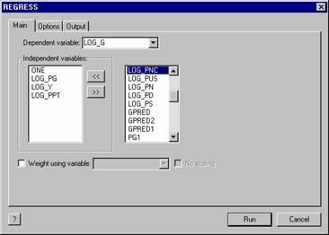
Models:Linear Models...:Regression, the dialog box presented is shown below.
On the main page, we
have selected the dependent variable (LOG_G) and the independent variables
(ONE, LOG_PG, LOG_Y, LOG_PPT). The
variable LOG_PNC is to be added to the list as well. The variable name is selected in the
right hand side window. Then, the << button is pressed to move
the name into the set of variables in the model. If you change your mind, you can move
variables back into the menu, out of the list by hightlighting in the left
hand side box and pressing the >>
button, instead.
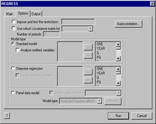
The Options page presents the extensions of the model, such as autocorrelation, panel data, and so on.
Autocorrelation is specified by pressing the button in
the options page. This opens the
dialog box shown at the right, where the estimator is selected.
![]()
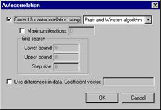
The autocorrelation dialog is concluded by pressing the OK button. Then, the model request can be submitted by pressing the Run button in the Regress window. The results will appear in the output, along with a copy of the command that is generated. If you wish to resubmit the model request with a small change, you can use Edit:Copy with Edit:Paste to put a copy of the command in your editing window, where you can edit it. (That is how we copied the command below, to our word processor.)
REGRESS;Lhs=LOG_G;Rhs=ONE,LOG_PG,LOG_Y,LOG_PPT,LOG_PNC;Ar1$
Note, finally, the question mark at the lower left of the dialog box. This invokes the Help file, and opens it to the chapter on the linear regression model.
B. The Scientific Calculator and Matrix Algebra
EA/LimDep's scientific calculator is an important tool. You can see an application in the example at the end of Section VII, where we used it to compute the F ratio for a Chow test, then looked up the 'p value' for the test by computing a probability from the F distribution. You can invoke the calculator with a CALC command that you put on your editing screen, such as CALC;1+1$, then highlight and submit with GO, as usual.

NOTE: CALC is a programming tool. As such, you will not always want to see the results of CALC. The CALC command above computes 1+1, but it does not display the result (2). If you want to see the result of CALC, add the word ;LIST to the command, as in CALC;LIST;1+1$
The one at the left shows
some of the range of calculations you can do with CALC; 1+1, the value of the standard normal density at x=0.3, the discounted present value
of a so called million dollar lottery paid out over 40 years, the 95th
percentile of the F distribution with 4 and 181 degrees of freedom, and,
finally, not shown yet, the 95th percentile of the standard
normal distribution. In addition
to the full range of algebra, CALC
The other way you can invoke the calculator is to use Tools:Scalar Calculator to open a calculator
window. This would appear like the one
below. When you use a window, the
results are always listed on the screen.
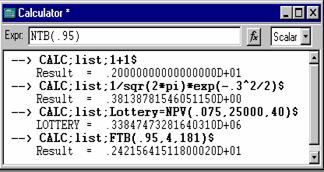
includes approximately 100 functions, such as the familiar ones, log, exp, abs, sqr, and so on, plus functions for looking up table values from the normal, t, F, and chi-squared distributions, functions for computing integrals (probabilities) from these distributions, and many other functions. You can find a full listing in Chapter 11 of the online manual.
Any result that you calculate with CALC can be given a name, and used later in any other context that uses numbers. Note, for example, in the third command, the result is called LOTTERY. All model commands, such as REGRESS, compute named results for the calculator. You can see the full list of these under the heading 'Scalars' in the project window shown in Section VII.B. above. After you use REGRESS to compute a regression, these additional results are computed and saved for you to use later. Note, once again, the example at the end of Section VII.H. Each of the three REGRESS commands is followed by a CALC command that uses the quantity SUMSQDEV. In each case, this value will equal the sum of squared residuals from the previous regression. That is how we accumulate the three values that we need for the Chow test. The other statistics, YBAR, LOGL, and so on, are also replaced with the appropriate values when you use REGRESS to compute a regression. The other model commands, such as PROBIT, also save these results, but in many cases, not all of them. For example, PROBIT does not save a sum of squared deviations, but it does save LOGL and KREG, which is the number of coefficients.
The NAMELIST command defines the matrices used. REGRESS
computes the residuals and calls them e. CREATE
uses the regression results. Finally, MATRIX does the
actual calculation. Discussion of the form of the matrix instruction
appears below.
The other
major tool you will use is the matrix algebra calculator. EA/LimDep
provides a feature that will allow you to do the full range of matrix algebra
computations used in the text, and far more. To see how this works, here is a fairly simple application: The LM statistic for testing the hypothesis
that
![]() =
= ![]() f(z g)
= s2
in a classical regression model is computed as LM = ½g Z(Z Z)-1Z g
where g is a vector of n observations on [ei2/(e e/n) - 1] with ei
the least squares residual in the regression of y on X, and Z is the set
of variables in the variance function. This instructions that would be used to compute this statistic:
f(z g)
= s2
in a classical regression model is computed as LM = ½g Z(Z Z)-1Z g
where g is a vector of n observations on [ei2/(e e/n) - 1] with ei
the least squares residual in the regression of y on X, and Z is the set
of variables in the variance function. This instructions that would be used to compute this statistic:
 Namelist
; X = the list of variables
; Z = the list of variables $
REGRESS ; Lhs = y ; Rhs = X ; Res = e $
CREATE ; g = (e^2/(sumsqdev/n)-1) $
MATRIX ; LM = .5 * g'Z * <Z'Z> * Z'g $
The MATRIX command works the same as CALC, either in the editor screen or in its own Tools window. The MATRIX feature in EA/LimDep is extremely large, and includes far too many features and extensions to list here. Chapter 10 of the online manual contains a full description of the command. There are applications that use matrix algebra throughout the rest of the manual.
There
are only a few things you need to get started using EA/LimDep's matrix algebra program. The first is how to define a data matrix, such as X in the example above. The columns of a data matrix are variables,
so, as you can see in the example, the NAMELIST
command defines the columns of a data matrix. A single variable defines a data
matrix with one column (i.e., a data vector) - note the use of the variable g in the example. The rows of a data matrix are the
observations in the current sample, whatever that happens to be at the
time. That means that all data matrices
change when you change the sample. For
example, NAMELIST;X=ONE,GNP,CPI,MONEY$
followed by SAMPLE;1-20$ defines a
20![]() 4 data matrix, but if you then give the command SAMPLE;11-20$, then X now has only 10 rows. Second, data matrices can share columns. For example, with the X just defined, we might also have a NAMELIST;Z=ONE,GNP,INFL,INTEREST$ Thus, X and Z share two columns. In matrix algebra,
the number 1 will represent a column
of ones. Thus, if x is a variable, you could compute its mean with MATRIX;List;Meanx=1/n*x'1$. There are many matrix operators. The major ones you need to know are (1) +, -,
* for the usual addition, subtraction, and multiplication - the program will
always check conformability, (2) ' (apostrophe) for transposition, and (3)
<.> for inversion. When you
compute a moment matrix, such as X X, you need not both transpose and multiply. The command X'X means exactly what it looks like. Finally, in order to define a matrix with
specific values in it, you use MATRIX;NAME
= [ row 1 / row 2 / ... ] $ Within a
row, values are separated by commas; rows are separated by slashes, and the
whole thing is enclosed in square brackets. An example appears below.
4 data matrix, but if you then give the command SAMPLE;11-20$, then X now has only 10 rows. Second, data matrices can share columns. For example, with the X just defined, we might also have a NAMELIST;Z=ONE,GNP,INFL,INTEREST$ Thus, X and Z share two columns. In matrix algebra,
the number 1 will represent a column
of ones. Thus, if x is a variable, you could compute its mean with MATRIX;List;Meanx=1/n*x'1$. There are many matrix operators. The major ones you need to know are (1) +, -,
* for the usual addition, subtraction, and multiplication - the program will
always check conformability, (2) ' (apostrophe) for transposition, and (3)
<.> for inversion. When you
compute a moment matrix, such as X X, you need not both transpose and multiply. The command X'X means exactly what it looks like. Finally, in order to define a matrix with
specific values in it, you use MATRIX;NAME
= [ row 1 / row 2 / ... ] $ Within a
row, values are separated by commas; rows are separated by slashes, and the
whole thing is enclosed in square brackets. An example appears below.
In the same way that every model command creates some scalar results, every model command also creates at least two matrices, one named B which is the coefficient vector estimated, and one called VARB which is the estimated covariance matrix. You can use these in your matrix commands just like any other matrix. For another example, here is a way to compute the restricted least squares estimator defined in Chapter 7 of the text, b* = b - (X X)-1R [R(X X)-1R ]-1(Rb - q). For a specific example, suppose we regress y on a constant, x1, x2, and x3, then compute the coefficient vector subject to the restrictions that b2 + b3 = 1 and b4 = 0. In a second example, we compute the Wald statistic for testing this restriction,
W = (Rb-q) [R s2(X X)-1R ]-1(Rb-q). Note that both examples use a shortcut for a quadratic form in an inverse, and the second example uses both B and VARB.


Namelist ; X = one,x1,x2,x3 $ NAMELIST ; X = one,x1,x2,x3 $
Regress ; Lhs = y ; Rhs = X $ Regress ; Lhs = y ; Rhs = X $
Matrix ; R = [0,1,1,0 / 0,0,0,1] ; q = [1/0] $ Matrix ; R = [0,1,1,0 / 0,0,0,1] ; q = [1/0] $
MATRIX ; m = R*b - q ; D = R*<X'X>*R' MATRIX ; m = R*b - q ; D = R*VARB*R'
; br = b - <X'X> * R'<D>m $ ; W = m' <D> m $
In addition to the operators and standard features of matrix algebra, there are numerous functions that you might find useful. These include ROOT(symmetric matrix), CXRT(any matrix) for complex roots (see Chapter 16 of the text for an application), DTRM(matrix) for determinant, SQRT(matrix) for square root, and a few dozen others. Chapter 10 of your online manual contains the full list of matrix functions.
Lastly, a special function, STAT(vector,matrix), is provided for you to display statistical results when you use matrix algebra (or any other means) to compute a coefficient vector and an associated asymptotic covariance matrix. To illustrate, we'll continue the example above. The asymptotic covariance matrix for the restricted least squares estimator is
Asy.Var[b*] = s*2
where s*2 = (y - Xb*) (y - Xb*)/(n-K-J) Here is a general program that could be used for this purpose. To adapt it to a specific problem, you'd need to define X and y and supply the particular R and q.

We do all computations using CREATE, CALC, and MATRIX
Namelist ; X = the set of variables $
CREATE ; y = the dependent variable $
Matrix ; R = the matrix of constraints (see Chapter 7 of the text)
; q = the vector on the RHS of the constraints $
MATRIX ; bu = <X'X> * X'y $
CREATE ; e = y - X'bu $
CALC ; K = Col(X) ; s2 = e'e/(n-K) ; J = Row(R) $
MATRIX ; Vb = s2 * <X'X> ; Stat (bu,Vbu) $ (Unrestricted)
MATRIX ; m = R*bu - q ; D = R*<X'X>*R'
; br = bu - <X'X>*R'<D>m
; Vbr = <X'X> - <X'X>*R'*<D>*R*<X'X> $
CREATE ; er = y - X'br $
CALC ; s2r = er'er / (n - K - J) $
MATRIX ; Vbr = s2r * Vbr ; Stat(br,Vbr) $
The program above is useful for seeing how MATRIX can be used to compute the restricted least squares estimator. It is also general enough that you can easily adapt it to any problem. But, for much greater convenience, since restricted linear regression is such a common application, the feature can be built into the REGRESS command, instead. To impose restrictions on a linear regression model, use this syntax:
Regress ; Lhs = ... ; Rhs = ...
; Cls: the restrictions, separated by commas if there are more than one $
with coefficients labeled b(1), b(2),... in the same order as the RHS variables. For the specific example above, the absolutely simplest way to obtain the restricted least squares estimates would be
(This can be done in the command builder dialog box, but it is not appreciably simpler to do it this way.) Restrictions must be specified linearly, without parentheses. Operations are only + and - and multiplication is implied. For example, CLS : 2b(1) + 3.14159b(4) - b(5) = 2 is a valid (if strange) constraint. Note that constraints must be in the form linear function = value, even if value is zero.
As discussed in Chapters 4, 9,
10, and elsewhere in the text, for a random vector b with estimated asymptotic covariance matrix,V, the estimated asymptotic covariance matrix for the set of
functions c(b) is GVG , where G
is the matrix of derivatives, ![]() c(b)/
c(b)/![]() b . This full
set of computations is automated for you in the WALD command. Generally, you
need only supply the vector and covariance matrix and a definition of the
function(s), and EA/LimDep computes G (by numerical approximation - see
Chapter 5 in the text) and the covariance matrix for you. For a regression model, it is even easier;
you need only supply the functions. The
command for WALD is
b . This full
set of computations is automated for you in the WALD command. Generally, you
need only supply the vector and covariance matrix and a definition of the
function(s), and EA/LimDep computes G (by numerical approximation - see
Chapter 5 in the text) and the covariance matrix for you. For a regression model, it is even easier;
you need only supply the functions. The
command for WALD is
WALD ; Start = b (the values of the coefficients)
; Var = V (the covariance matrix)
; Labels a set of names for the coefficients (like NLSQ defined earlier)
; Fn1 = first function ; ... $ (up to 5 functions).
This coefficient vector and covariance matrix may be any that are obtained from any previous operations.
For example, in Example 7.14 in the text, we estimated the parameters [a,b,g] in the consumption function Ct = a + bYt + gCt-1 + et. We then estimated the long run marginal propensity to consume, b/(1-g), which is a nonlinear function, and computed an estimate of the asymptotic standard error for this estimate. The text shows the computations, done 'the hard way.' Here is an easier way to compute the long run MPC and estimate the asymptotic standard error:
REGRESS ; Lhs = C ; Rhs = One,Y,Clag $
WALD ; Start = B ; Var = VARB
; Labels = alpha,beta,gamma ; Fn1 = beta/(1-gamma) $
This computes the function and also estimates and reports the standard error and an asymptotic 't-ratio.' In fact, if you are analyzing the coefficients of an immediately preceding regression , there is yet a shorter way. The following is equivalent to the WALD command above:
When you use the syntax B_Variable name, EA/LimDep understands this to have been constructed from a previous regression, and builds up the function and the results using B and VARB from that regression.
WALD also tests linear or nonlinear hypotheses. It automatically computes the WALD statistic for the joint hypothesis that the functions are jointly zero. For two examples, in the preceding, to test the hypothesis that the long run MPC equals 1.0, you would use WALD ; Fn1 = B_Y / (1 - B_CLAG) - 1 $ Second, for the Wald test that we did in the matrix algebra section above, we could have used
REGRESS ; Lhs = Y ; Rhs = One,x1,x2,x3 $
WALD ; Fn1 = B_X1 + B_X2 - 1 ; Fn2 = B_X3 $
The last (and most advanced) tool we will examine is the procedure. A procedure is a group of commands that you can collect and give a name to. Then, to execute the commands in the procedure, you simply use an EXECUTE command. To define a procedure, just place the group of commands in your editor window between PROCEDURE=the name$ and ENDPROCEDURE$ commands, then Run the whole group of them. They will not be carried out at that point; they are just stored and left ready for you to use later. For example, the application above that computes a restricted regression and reports the results could be made into a procedure as follows:
Namelist ; X = the set of variables $
CREATE ; y = the dependent variable $
Matrix ; R = the matrix of constraints (see Chapter 7 of the text)
; q = the vector on the RHS of the constraints $
PROCEDURE = CLS $
... the rest of the commands above
ENDPROCEDURE $
Now, to compute the estimator, we would define X, y, R, and q, then use the command
EXECUTE ; Proc = CLS $
To use a different model, we'd just redefine X, y, R, and q, then execute again. Since the commands for this procedure are just sitting on the screen waiting for us to Run them with a couple of mouse clicks, this really has not gained us very much. There are two better reasons for using procedures. First, the EXECUTE command can be made to request more than one run of the procedure, and, second, procedures can be written with 'adjustable parameter lists,' so that you can make them very general, and can change the procedure very easily. We'll consider one example of each.
The following computes bootstrap standard errors for least squares. (This will introduce a new command, the DRAW command to sample from the current sample.) Bootstrapping is described in Chapter 5 of the text, and applied in Chapter 10, so, we'll just proceed to the application:

NAMELIST ; X = the independent variables $
CREATE ; y = the dependent variable $
MATRIX ; b0 = <X'X> * X'y $
CALC ; K0 = Col(X) ; NREP = 100 $
MATRIX ; Vb0 = 0.0[K0,K0] $
CALC ; CurrentN = N $
PROCEDURE = Boot $
DRAW ; N = CurrentN ; Replacement $
MATRIX ; dr = <X'X> * X'y - b0
; Vb0 = Vb0 + 1/NRep * dr * dr' $
ENDPROC $
EXECUTE ; Proc = Boot ; N = NRep $
MATRIX ; Stat (b0,Vb0)$
For our second and final example, we'll construct a procedure for doing a Chow test of structural change based on an X matrix, a y variable, and a dummy variable, d, which separates the sample into two subsets of interest. We'll write this as a 'subroutine' with adjustable parameters. This is how a such a procedure that might be included as an appendix in an article would appear. Note that this routine does not actually report the results of the three least squares regressions. To add this to the routine, the CALC commands which obtain sums of squares could be replaced with REGRESS ;Lhs = y ; Rhs = X $ then CALC ; ee = sumsqdev $

/* Procedure to carry out a Chow test of structural change.
Inputs: X = namelist that contains full set of independent variables
y = dependent variable
d = dummy variable used to partition the sample
Outputs F = sample F statistic for the Chow test
*/ F95 = 95th percentile from the appropriate F table.
PROC = ChowTest(X,y,d) $
CALC ; K = Col(X) ; Nfull = N $
SAMPLE ; All $
CALC ; ee = Ess(X,y) $
INCLUDE ; New ; D = 1 $
CALC ; ee1 = Ess(X,y) $
INCLUDE ; New ; D = 0 $
CALC ; ee0 = Ess(X,y) $
CALC ; List ; F = ((ee-(ee1+ee0))/K) / (ee/(Nfull-2*K) )
; F95 = Ftb(.95,K, (Nfull-2*K)) $
ENDPROC
Now, suppose we wished to carry out the test of whether the labor supply behaviors of men and women are the same . The commands might appear as follows:
NAMELIST ; HoursEqn = One,Age,Exper,Kids $
EXECUTE ; Proc = ChowTest(HoursEqn,Hours,Sex) $
|