Fighter Jet Vectoring Nozzle

In this exercise, we will perform a structural analysis of a vectoring nozzle used on a high performance jet fighter engine. Today's state-of-the-art fighter aircraft are using vectoring nozzle technology to gain a performance edge over the competition. Airplanes are propelled forward by the expulsion of exhaust from the engine. Thrust vectoring is a method of changing the exhaust in a way that would cause the aircraft to change direction in a more abrupt manner than can be done with traditional control surfaces such as flaps (ailerons, elevators, and rudders).

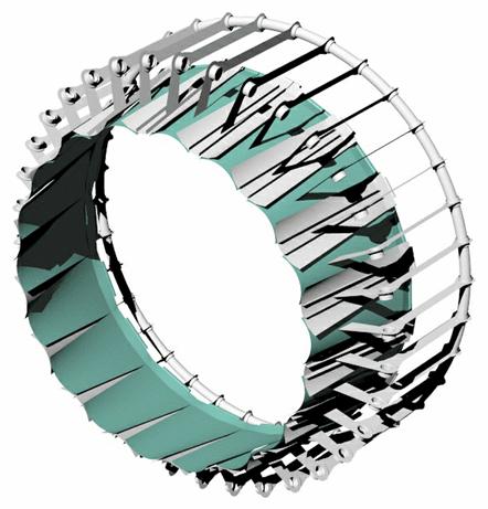
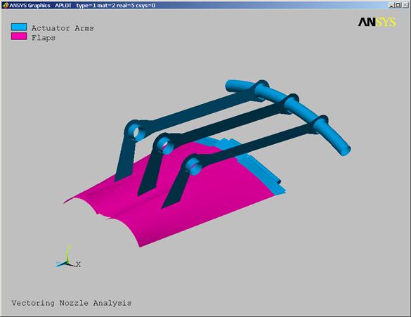
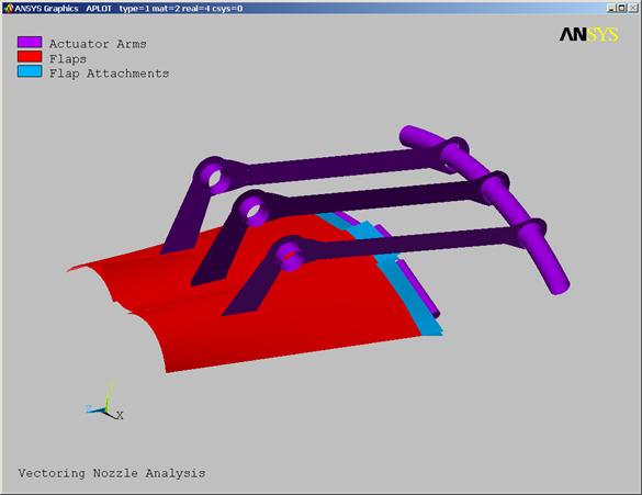
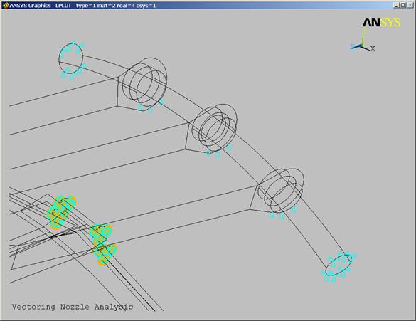
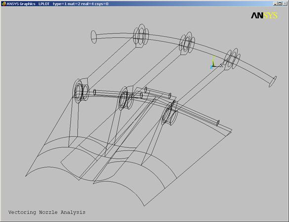
The nozzle design in this exercise (figure below) is similar in concept to one used in a current jet fighter engine in service today. It consists of a series of flaps hinged to a ring (A) at the forward section, and connected to a secondary outer ring (B) through a set of struts (C). Moving the outer ring forward or backwards controls the throat area of the nozzle. Vectoring is accomplished by tilting the outer ring, or moving it up/down/left/right relative to the engine axis. These movements are controlled by a series of actuator arms connected to the outer ring (not shown).

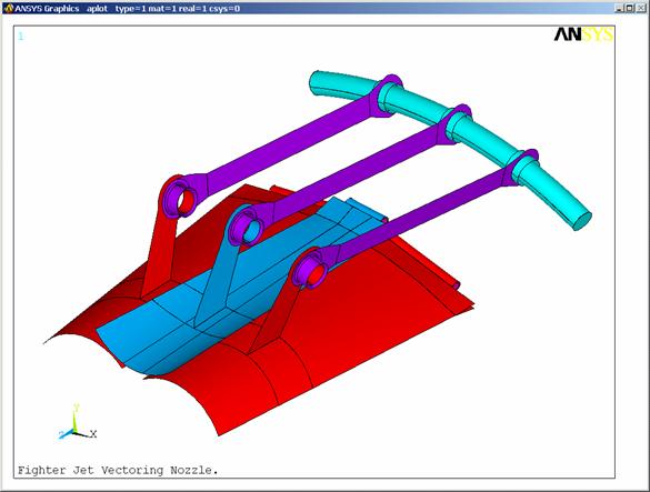
The nozzle is a complex assembly of several parts acting together. The goal of this analysis is to demonstrate ANSYS/Professional's ability to recognize assemblies, and automatically detect and correctly model all contact surfaces with nonlinear surface-to-surface contact elements. We will then use this model to determine the stresses and deflections of the nozzle under the extreme conditions experienced during an air-to-air combat mission. We will use symmetry to our advantage and model a 3-flap segment of the full nozzle.

The ANSYS/Professional MTB will be used to import the shell model. The AutoContact feature will be used to automatically detect and model the assembly interfaces with contact elements.

The assembly/contact capability of ANSYS/Professional will be explained in this exercise. Basic Mechanical Toolbar interaction is explained in detail in Exercise 1, which we recommend completing before starting this exercise.

Summary of steps:

Launch ANSYS/Professional

Launch ANSYS using your start menu

Mechanical Toolbar Setup:

Toolbar settings

Model:

Import Model

Assign Thicknesses

Material Properties

Contact Definition

Meshing

Loads:

Hinge Constraints

Actuator Arm Displacements

Pressure Loads

Solve

Save Model

Perform Solution

Post Processing

Stress Plots

Query Results

Animate Results

Report Generation

Conclusions:

Exit ANSYS.

Step-by-step Instructions:

Before beginning this problem, create a separate folder on your computer for this job and copy the ANSYS database nozzlegeom.db to this folder from the CD.

Launch ANSYS/Professional

Launch ANSYS using your start menu

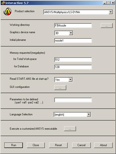
A. Browse to select the working directory you just c 11411d34l reated for this job.

B. Enter a job name (nozzle1). All ANSYS files created for this problem will have a filename of nozzle1 followed by a unique extension.

C. Change the workspace and database sizes for this job to be 512 and 128 respectively.

D. Click RUN to start the ANSYS GUI.

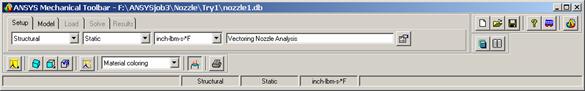
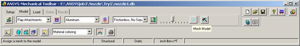
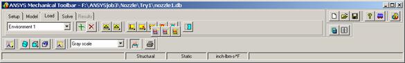
Mechanical Toolbar Setup

Toolbar settings.

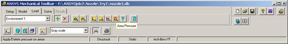
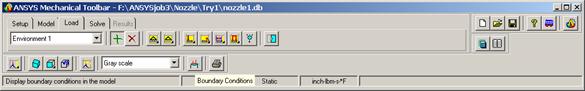
A. Change the units to inch-lbm-s-F

B. Change the title to Vectoring Nozzle Analysis

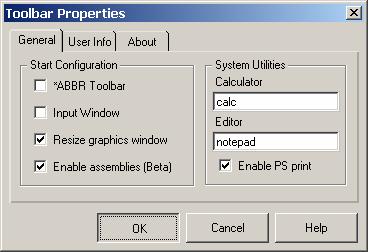
C. Pick the Toobar Properties button

D. A Toolbar Properties dialog will appear. Check the Enable assemblies option. This activates the feature that automatically detects and creates contact surfaces. Note: You may not see this option depending on the version of ANSYS you are running.

E.

OK

Model

Import Model.

A. Pick the Model tab in the Mechanical Toolbar (MTB).

B. Next, we will import the Nozzle geometry from an ANSYS database. (ANSYS can import a variety of geometry formats as well). Pick the Import Geometry button.

C. A dialog box will appear for you to select the file to import. Change the Files of type setting to ANSYS (*db)

D. Select nozzlegeom.db

E.

Open.

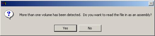
F. Ansys will ask if you want to import this model as an assembly. Pick Yes.

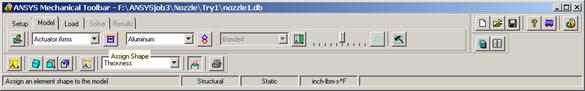
Assign Thicknesses:

A. ANSYS will prompt you for a set of default shell element properties for the model. Enter a name of Actuator Arms, and a thickness of 0.10.

B. OK.

C. Our assembly will have three unique shell thicknesses. Let's first assign the Actuator Arms property to the entire model, and then modify the other two properties afterwards. Pick the Assign Shape button.

D. A dialog box will appear for you to select areas to assign this property to. Click the Pick All button.

E. Next, we will define a thickness for the flaps. In the default shapes list, pick Shell.

F. A dialog will appear for you to define a new shell property. Enter Flaps for the name, and 0.05 for the thickness.

G.

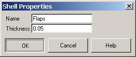
Pick OK.

H. Pick the Assign Shape button again to assign this property to the flaps.

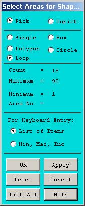
I. A dialog box appears for you to select the areas to assign the flap property to. Change the method of selection from single to loop. This method selects all areas that form a continuous connection and is an easy way to select all areas on a part.

J.

Pick one area on each of the three flaps. ANSYS should select all areas on each flap for a total of 19 areas.

K. Note the total selected areas should be 19. Pick OK.

L. The plot should change to color the areas based on the properties we have defined so far.

M. Let's repeat this procedure to define a thickness for the flap attachments. Pick Shell in the

Default Shape list.

N. For the property name, enter Flap Attachment, and for the thickness enter 0.20.

O.

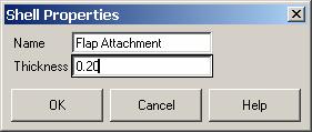
OK.

P. To assign the next property, it may be easier to view lines instead of areas. Click and hold the plot button until the flyout appears and pick the plot lines button.

Q. Pick the Assign Shape button.

R. Pick the areas at the rear of each flap that connect to the hinge cylinders. There should be a total of 8 areas. You may have to use the pan/zoom/rotate function to obtain a better view.

S. OK.

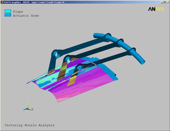
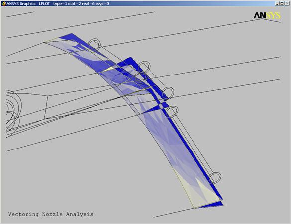
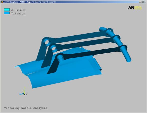
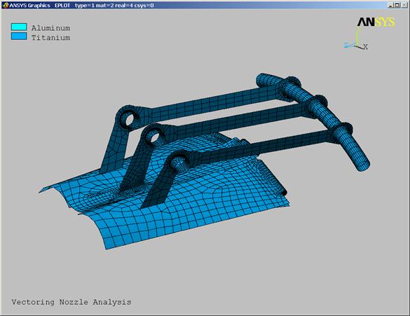
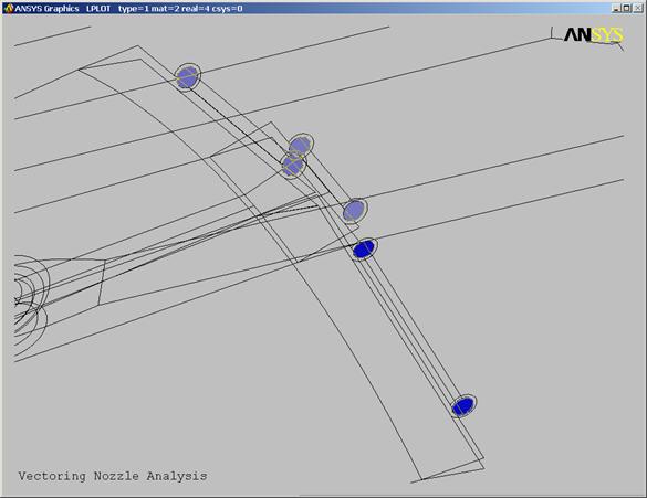
T. ANSYS will replot your model highlighting all the thickness assignments. It should look like the plot below.

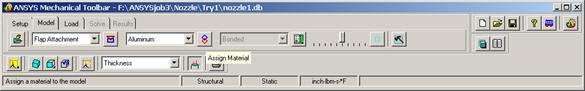
Material Properties.

A. Next, we need to assign this material to the model. Pick the Assign Material button.

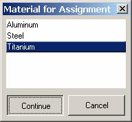
B. A dialog box will appear for you to select a material. Pick Titanium.

C. Continue.

D. In the Select Areas for Material dialog, click the Pick All button

E. Your model should now be color coded to indicate it is all titanium.

Contact Definition:

A. We are ready to define the contact surfaces. ANSYS can automatically detect areas that are in or near contact and define contact pairs. Click and hold the View/Modify Contact button until the fly-out appears. Pick the Auto Create Contact button.

B.

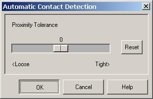
ANSYS will search for surfaces that are within a certain proximity to each other when defining contact pairs. A proximity tolerance of 1 (Tight) means that surfaces must be exactly touching in order for contact to be defined. For our model, use the default tolerance. Pick OK. ANSYS will create the contact pairs. This may take a few minutes.

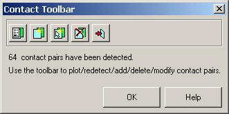
C. When ANSYS finishes, a dialog will appear indicating that 64 contact pairs have been created. This dialog contains several options as shown below.

D. Pick the View/Modify Contact button.

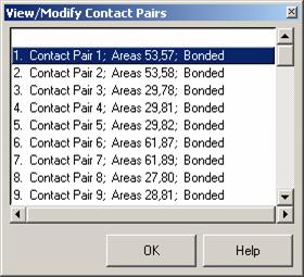
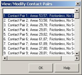
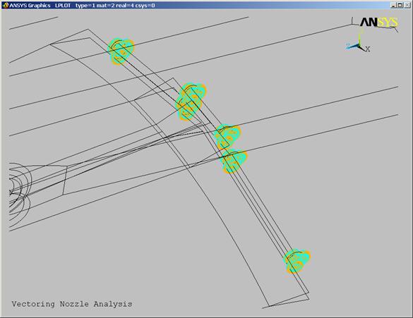
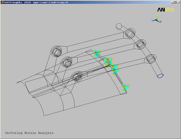
E. A dialog will appear with all the contact surfaces listed. The first pair will be highlighted and shown in graphics window.

F. In the View/Modify Contact Pairs dialog, click on Contact Pair 3.

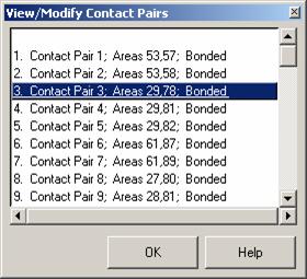
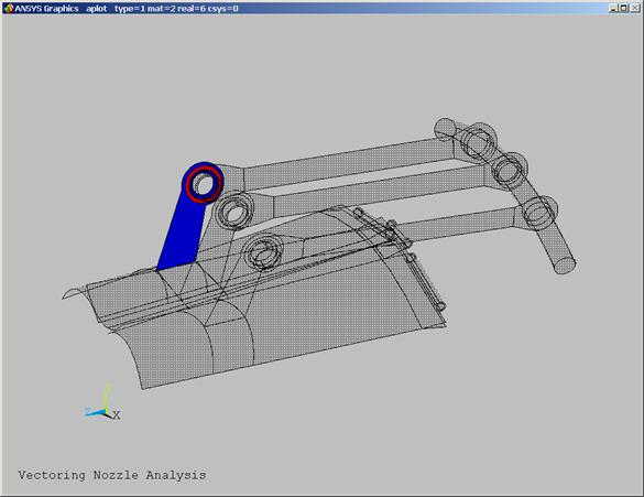
G. This pair will be highlighted in the graphics window.

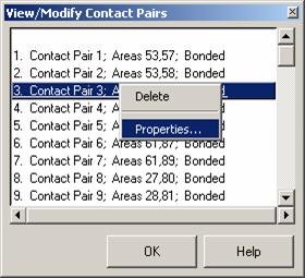
H. With your mouse in the View/Modify Contact Pairs dialog, click the right mouse button.

	Right click mouse with cursor in this dialog. Right click mouse with cursor in this dialog.

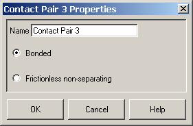
I. An option will appear for you to delete this pair, or modify its properties. Pick the Properties button.

J. You can modify the name for this contact pair to be something more descriptive if you like. Also, you can choose between bonded or Frictionless non-separating behavior. Bonded is useful for "welding" two parts together that have dissimilar meshes. For our model, we want to change all contact surfaces to be frictionless non-separating. We could change them here, but we would have to do each one individually. There is an easier way. Pick Cancel to close this dialog.

K.

Pick OK to close the View/Modify Contact Pairs dialog.

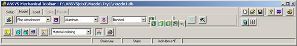
L. Pick the Default Contact Properties arrow in the MTB and change the Bonded behavior to Frictionless No Separation

M. Pick the View/Modify Contact fly-out button.

N. All contact pairs should now indicate Frictionless Sliding contact. Pick OK to close the View/Modify Contact Pairs dialog.

Meshing:

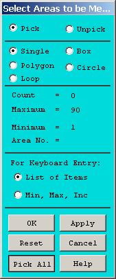
A. We are now ready to mesh our model. We will use the default smart size settings. Pick the Mesh Model button.

B. In the Select Areas for Meshing dialog, click the Pick All button. This may take a few minutes. ANSYS will mesh the entire assembly.

C. When completed, ANSYS will replot the areas. Use the Plot flyout to plot elements.

Loads:

We are now ready to apply loads and boundary conditions to our model. These will consist of fixing the ends of the hinge pins against all motion, displacing the ends of the actuator ring up and backwards, and applying a pressure load to the internal surfaces of the flaps.

Hinge Constraints:

A. First, we must enter the Loads module. In the MTB, pick the Load tab.

B. For this operation, it will be easier to apply loads if our graphics plot is in the line mode. Use the plot flyout to plot lines.

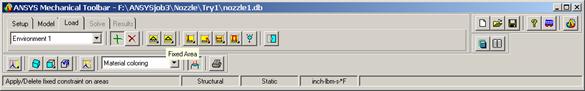
C. Pick the Fixed Area button.

D.

Use the pan/zoom/rotate function to zoom in on the flap hinge area. Pick the areas on the ends of each of the hinges. There should be six total.

E. OK.

F. ANSYS will draw fixed constraint symbols on these areas.

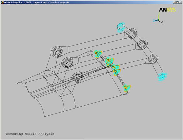
Actuator Arm Displacements

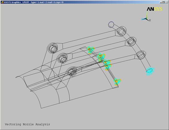
A. Use the fit button in the pan/zoom/rotate function to restore the view to the full model. We will now apply the actuator arm displacements to the cut ends of the actuator ring. Since the ring is hollow, we do not have an area at the cut ends to apply displacements too. We have to apply the displacements to the circular lines. In the MTB, click and hold the area displacement button until the flyout appears. Pick the Displaced Line button.

B.

A dialog box will appear for you to select the lines. Pick the two lines that make up the ends of the actuator arm closest to you.

C. 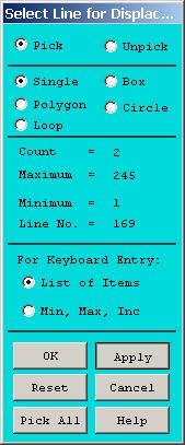Apply.

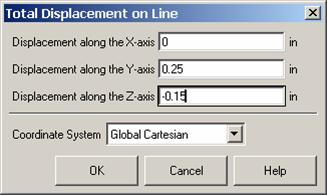
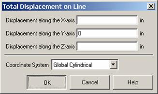
D. A dialog will appear for you to enter the displacements. Note the coordinate system triad in the upper right corner of your graphics window. Enter the three displacements as shown below.

E. OK.

F. Constraint symbols should appear on the lines.

G. The select lines for displacement dialog should still be open. Pick the two lines on the other side of the actuator ring.

H.

Apply.

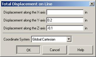
I. Enter the displacements shown in the Total Displacement on Line dialog box.

J.

OK.

K. The fixed displacements should be plotted in the graphics window as shown below.

L.

We also need to apply some constraints to the actuator arms in the circumferential direction in order to prevent rigid body motion. Pick one of the circular lines on each of the three actuator arms where they attach to the ring as shown below.

M. 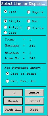OK.

N. For Displacement along the Y-axis, enter zero.

O. Use the scroll arrow to select Global Cylindrical for the Coordinate System. This system is oriented such that the global Z-direction is the axis of rotation, X is radial, and Y is along the circumference.

P. OK.

Q. ANSYS will apply symbols to the lines as shown. The symbol direction will show constraints in the vertical direction instead of the desired circumferential direction. These loads will be oriented correctly during solution when they are transferred from the geometry to the finite element mesh.

Pressure Loads:

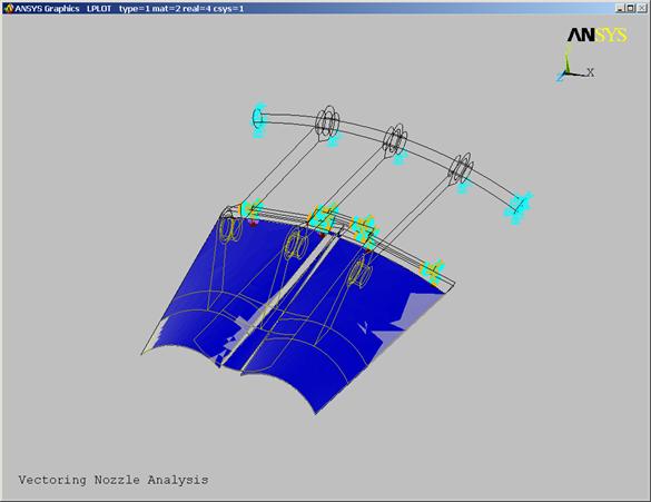
A. We have completed application of the constraints and enforced displacements. Next, we will apply the pressure loads on the interior of the flaps. In the MTB, pick the Area Pressure button.

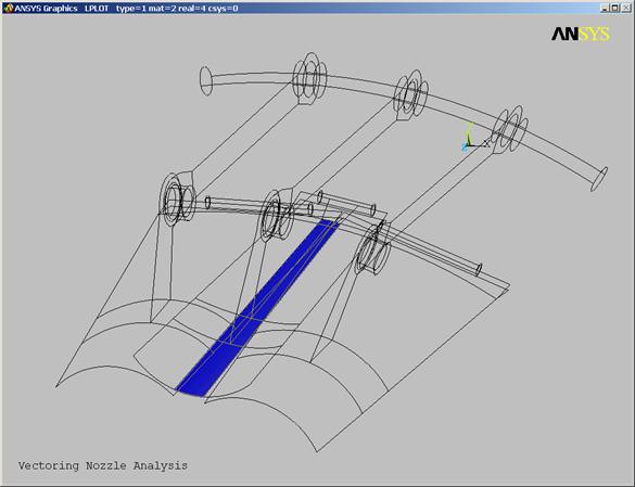
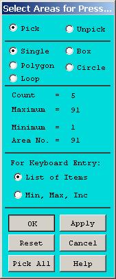
B. A dialog box will appear for you to select areas for pressure loading. We will apply a 15-PSI pressure load to the internal surfaces of the flaps. Note that the center flap will only have pressure on the center strip of areas since the edges of this flap are sealed against the outer flaps. We will start by selecting these center flap areas. Using the dynamic viewing controls, orient your view as shown below and pick the center areas of the center flap. You should pick a total of 5 areas.

Hint: If you click and hold the left mouse button while dragging across the screen, each area to be selected will be highlighted. The area is not actually selected until you release the button. If you accidentally select a wrong area, click the right mouse button. The cursor will change from an upward pointing arrow to a downward pointing arrow indicating that you can now unpick items from the selection with the left mouse button. Click the right button again to toggle back to picking.

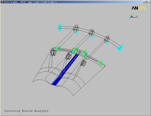
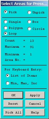
C. With the center flap areas still highlighted, change the method of selection from Single to Loop

D. Pick one area on each of the outer flaps. ANSYS should loop through and select all areas on these two flaps.

E. Note in the select areas dialog, you should have a total of 13 areas selected.

F. Pick OK.

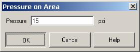
G. A dialog will appear for you to enter the pressure. Enter 15.

H. OK.

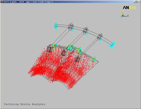
Hint: When working with shell elements, positive pressure loads act on the "top" face of the element. This orientation is determined by the element normal direction, which in turn is determined by the orientation of the area that the elements belong to. Since we have no way to control this in our model, it is easiest to just guess at a positive or negative sign, apply the loads and see what happens. ANSYS will draw arrows indicating the direction the loads act. If we guess incorrectly, just reapply the loads again changing the sign of the pressure. The new loads will overwrite the old ones.

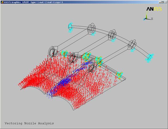
I. ANSYS will plot the loads as shown below.

J. Use the pan/zoom/rotate function to select a front view and scrutinize all areas of the model. Note that the pressure loads on the center flap are oriented inward in the wrong direction. We will have to reapply this pressure with a negative value.

K. Pick the Area Pressure button again.

L. To aid in selecting the areas, use the dynamic viewing controls to orient your view as shown below.

M.

Pick the Boundary Conditions button to turn off the pressure arrows.

N. As we did before, pick the five areas on the center of the center flap.

O.

Count should be 5.

OK.

P. Enter a value of -15.

Q. OK.

R. ANSYS will reapply the pressure load to the model. You may have to pick the Boundary Conditions button again to turn the pressure arrows back on.

S. Use the dynamic viewing controls to verify that all pressure load areas are pointing in the correct direction now. Note that the arrow color may have changed from red to blue, but the arrow direction is the important indicator.

Solve:

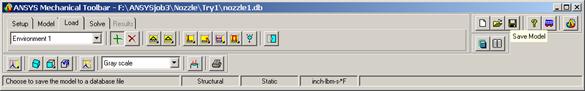
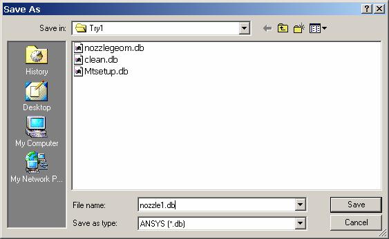
Save Model.

A. We have completed the modeling process and are ready to solve the problem. Before we proceed, let's save our work. Pick the Save button.

B. A dialog will appear for you to enter a database name to save to. Enter nozzle1.db.

C. Save.

Perform Solution:

A. Pick the Solve tab in the MTB.

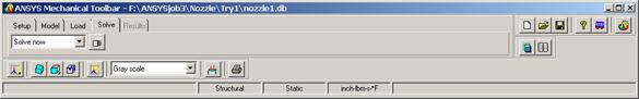
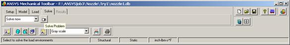
B. Pick the Solve Problem button.

C.

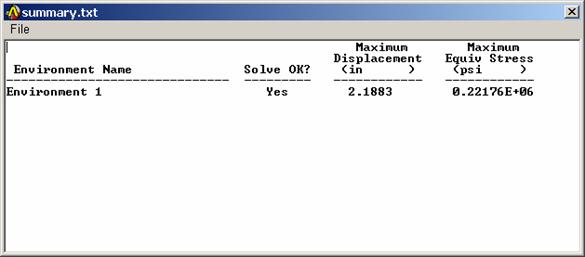
It will take ANSYS several minutes to solve this problem. When it is completed, a list window will appear with a summary of the max stress and displacement as shown below (your values may be slightly different). Close the summary.txt listing when you are through looking at it.

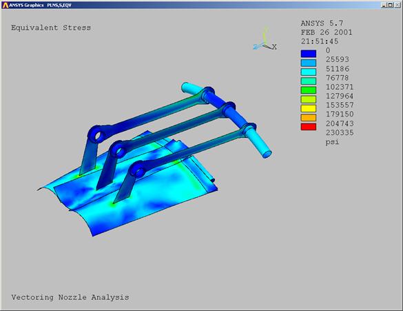
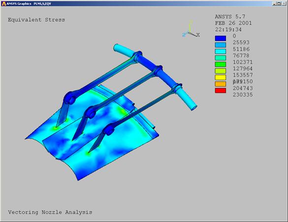
D. ANSYS will also display a von Mises stress plot of the model in the graphics window.

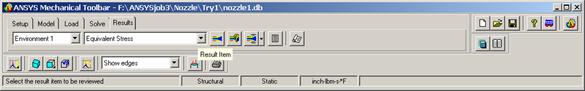
Post Processing:

Stress Plots.

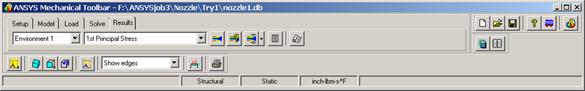
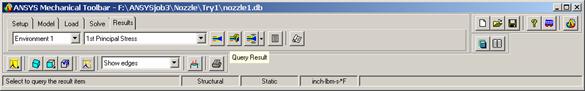
A. The Results Tab will now be activated in the MTB. Change the Results Item from Equivalent Stress to 1^st Principal.

B. Pick the Plot Result button.

C. The Maximum Principal stress will be displayed in the graphics window.

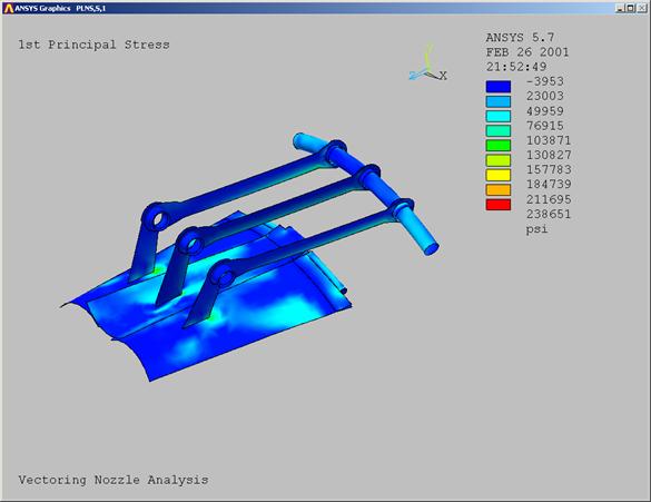
D.

Using the pan/zoom/rotate function, zoom in on the center flap/strut joint as shown below:

Query Results:

A. Pick the Query Result button in the MTB.

B.

Hold the left mouse button down and drag the cursor across the screen. The Max Principal stress value will be shown as you mouse over each node. Release the mouse button as you pick the node at the rear intersection of the center flap and strut as shown below:

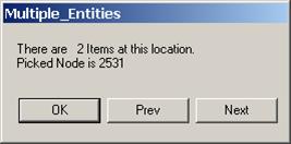
C. A warning will pop up that there are two items at this location. Since this node is connected to elements in both the flap and the strut, there are stress values associated with it from both parts. Pick the Next button to display the other stress result at this node.

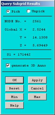
D.

With the maximum value displayed in the graphics window, pick the OK button. Is this maximum stress on the flap or the strut? The stress contour plot should indicate to you that the maximum stress is on the flap.

E. In the Query Subgrid Results dialog, pick the generate 3D Anno button.

F. OK.

G.

ANSYS will annotate the plot with an arrow and stress value pointing to this node. This will aid you in creating professional looking graphics for your reports.

Animate Results:

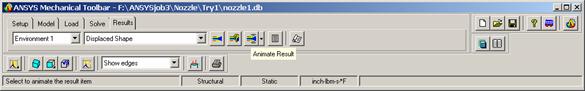
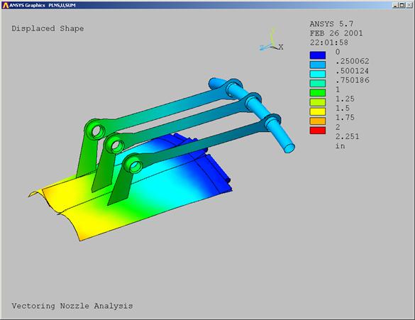
A. Next, let's animate the total displaced shape. In the Results Item scroll list, pick Displaced shape.

B. Before we start the animation, use the pan/zoom/rotate dialog to fit the model to the view. Then, pick the Animate Results button.

C. ANSYS will generate an animation of the total displacement. Pick the image below for an example.

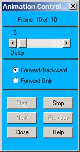
D.

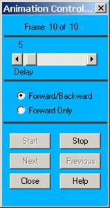
When you are through viewing this animation, pick the Close button in the Animation Control dialog.

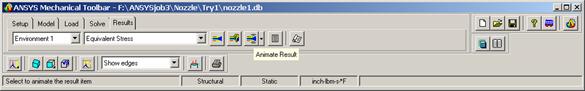
E. Let's repeat this procedure and animate the von Mises stress results as well. In the Results Item list, select Equivalent Stress.

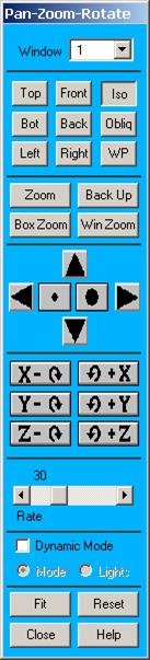
For a different perspective, use the pan/zoom/rotate function to select the Front view.

F. 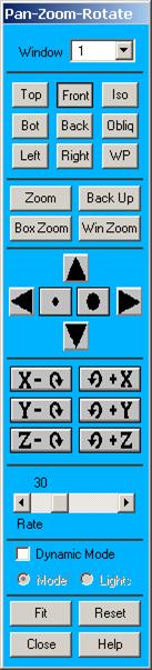Pick the Animate Results button again.

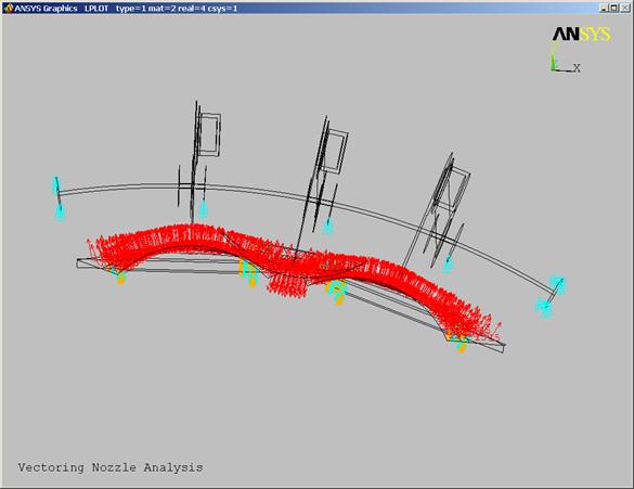
G. With this engine axis view, we can see how the nozzle flaps open to vector the thrust upwards.

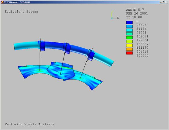
H. Close the animation when you are through viewing it.

I. Use the pan/zoom/rotate function to select an isometric view. Pick the Iso button.

J. The isometric view should look like this.

Report Generation:

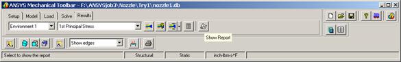
A. Let's generate an HTML report of our results. Pick the Show Report button in the MTB.

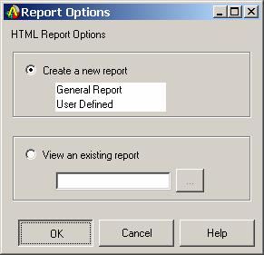
B. The default setting is to generate a new report. Pick OK.

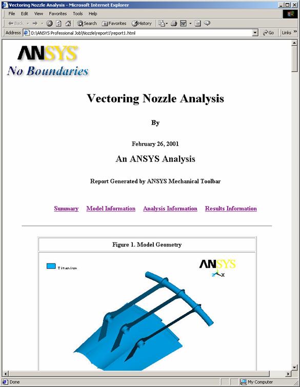
C. It may take a few minutes. When completed, ANSYS will launch the report in your default Internet browser. Pick the image below for a sample report.

Conclusions:

We have completed our analysis. What have we learned about the nozzle assembly? The stress level in the flaps appears to be too high. How could we reduce this stress? A thickness change from 0.050 to 0.075 would lower the stress significantly, however what would this do to the weight of our nozzle? What other alternatives are there? A honeycomb pattern of stiffening ribs would lower the stress level without increasing the weight as much as a change in thickness.

Exit Ansys:

A. We have completed our analysis. Exit ANSYS by picking: File >Exit.

B. Quit - No save!

C.

OK.